Content from Python Fundamentals

---

Last updated on 2025-10-13 | Edit this page

Estimated time: 30 minutes

Overview

Questions

• “What basic data types can I work with in Python?”
• “How can I create a new variable in Python?”
• “Can I change the value associated with a variable after I create it?”
• “How do I use a function?”

Objectives

• “Perform simple calculations.”
• “Assign values to variables.”
• “Understand the difference between int, float and str data types.”
• “Use the print and type built-in functions.”

Variables

---

Python can be used as a calculator:

PYTHON

3 + 5 * 4

OUTPUT

23

This is great but not very interesting. To do anything useful with data, we need to assign its value to a variable. In Python, we can assign a value to a variable using the equals sign =. For example, we can track the weight of a patient who weighs 60 kilograms by assigning the value 60 to a variable weight_kg:

PYTHON

weight_kg = 60

From now on, whenever we use weight_kg, Python will substitute the value we assigned to it. In layperson’s terms, a variable is a name for a value.

In Python, variable names:

• can include letters, digits, and underscores
• cannot start with a digit
• are case sensitive.

This means that, for example:

• weight0 is a valid variable name, whereas 0weight is not
• weight and Weight are different variables

Types of data

---

Python knows various types of data. Three common ones are:

• integer numbers
• floating point numbers, and
• strings.

In the example above, variable weight_kg has an integer value of 60. If we want to more precisely track the weight of our patient, we can use a floating point value by executing:

PYTHON

weight_kg = 60.3

To create a string, we add single or double quotes around some text. To identify and track a patient throughout our study, we can assign each person a unique identifier by storing it in a string:

PYTHON

patient_id = '001'

Using Variables in Python

---

Once we have data stored with variable names, we can make use of it in calculations. We may want to store our patient’s weight in pounds as well as kilograms:

PYTHON

weight_lb = 2.2 * weight_kg

We might decide to add a prefix to our patient identifier:

PYTHON

patient_id = 'inflam_' + patient_id

Built-in Python functions

---

To carry out common tasks with data and variables in Python, the language provides us with several built-in functions. To display information to the screen, we use the print function:

PYTHON

print(weight_lb)
print(patient_id)

OUTPUT

132.66
inflam_001

When we want to make use of a function, referred to as calling the function, we follow its name by parentheses. The parentheses are important: if you leave them off, the function doesn’t actually run! Sometimes you will include values or variables inside the parentheses for the function to use. In the case of print, we use the parentheses to tell the function what value we want to display. We will learn more about how functions work in later episodes.

We can display multiple things at once using only one print call:

PYTHON

print(patient_id, 'weight in kilograms:', weight_kg)

OUTPUT

inflam_001 weight in kilograms: 60.3

We can also call a function inside of another function call. For example, Python has a built-in function called type that tells you a value’s data type:

PYTHON

print(type(60.3))
print(type(patient_id))

OUTPUT

<class 'float'>
<class 'str'>

Moreover, we can do arithmetic with variables right inside the print function:

PYTHON

print('weight in pounds:', 2.2 * weight_kg)

OUTPUT

weight in pounds: 132.66

The above command, however, did not change the value of weight_kg:

PYTHON

print(weight_kg)

OUTPUT

60.3

To change the value of the weight_kg variable, we have to assign weight_kg a new value using the equals = sign:

PYTHON

weight_kg = 65.0
print('weight in kilograms is now:', weight_kg)

OUTPUT

weight in kilograms is now: 65.0

Variables as Sticky Notes

---

A variable in Python is analogous to a sticky note with a name written on it: assigning a value to a variable is like putting that sticky note on a particular value.

Using this analogy, we can investigate how assigning a value to one variable does not change values of other, seemingly related, variables. For example, let’s store the subject’s weight in pounds in its own variable:

PYTHON

# There are 2.2 pounds per kilogram
weight_lb = 2.2 * weight_kg
print('weight in kilograms:', weight_kg, 'and in pounds:', weight_lb)

OUTPUT

weight in kilograms: 65.0 and in pounds: 143.0

Similar to above, the expression 2.2 * weight_kg is evaluated to 143.0, and then this value is assigned to the variable weight_lb (i.e. the sticky note weight_lb is placed on 143.0). At this point, each variable is “stuck” to completely distinct and unrelated values.

Let’s now change weight_kg:

PYTHON

weight_kg = 100.0
print('weight in kilograms is now:', weight_kg, 'and weight in pounds is still:', weight_lb)

OUTPUT

weight in kilograms is now: 100.0 and weight in pounds is still: 143.0

Since weight_lb doesn’t “remember” where its value comes from, it is not updated when we change weight_kg.

Comments in Python

---

Everything in a line of code following the ‘#’ symbol is a comment that is ignored by Python. Comments allow programmers to leave explanatory notes for other programmers or their future selves.

Challenge

Check Your Understanding

What values do the variables mass and age have after each of the following statements? Test your answer by executing the lines.

PYTHON

mass = 47.5
age = 122
mass = mass * 2.0
age = age - 20

Show me the solution

OUTPUT

`mass` holds a value of 47.5, `age` does not exist
`mass` still holds a value of 47.5, `age` holds a value of 122
`mass` now has a value of 95.0, `age`'s value is still 122
`mass` still has a value of 95.0, `age` now holds 102

Challenge

Seeing Data Types

What are the data types of the following variables?

PYTHON

planet = 'Earth'
apples = 5
distance = 10.5

Show me the solution

PYTHON

print(type(planet))
print(type(apples))
print(type(distance))

OUTPUT

<class 'str'>
<class 'int'>
<class 'float'>

Key Points

• “Basic data types in Python include integers, strings, and floating-point numbers.”
• “Use variable = value to assign a value to a variable in order to record it in memory.”
• “Variables are created on demand whenever a value is assigned to them.”
• “Use print(something) to display the value of something.”
• Functions take zero or more parameters that send a value or variable to the code in the function to use.
• “Built-in functions are always available to use.”

Content from Loading and Analyzing Argo Float Data

---

Last updated on 2025-10-14 | Edit this page

Estimated time: 30 minutes

Overview

Questions

• “How can I process tabular data files in Python?”

Objectives

• “Explain what a library is and what libraries are used for.”
• “Import a Python library and use the functions it contains.”
• “Read tabular data from a file into a program.”
• “Select individual values and subsections from data.”
• “Perform operations on arrays of data.”

Words are useful, but what’s more useful are the sentences and stories we build with them. Similarly, while a lot of powerful, general tools are built into Python, specialized tools built up from these basic units live in libraries that can be called upon when needed.

Loading data into Python

---

To begin processing the Argo data, we need to load it into Python. We can do that using a library called NumPy, which stands for Numerical Python. In general, you should use this library when you want to do fancy things with lots of numbers, especially if you have matrices or arrays. To tell Python that we’d like to start using NumPy, we need to import it:

PYTHON

import numpy

Importing a library is like getting a piece of lab equipment out of a storage locker and setting it up on the bench. Libraries provide additional functionality to the basic Python package, much like a new piece of equipment adds functionality to a lab space. Just like in the lab, importing too many libraries can sometimes complicate and slow down your programs - so we only import what we need for each program.

Before we load any data it can be helpful to tell NumPy not to print all the lines in our data since some of our data is quite big and we probably don’t want to see every line of it. NumPy includes a function called set_printoptions which we can use to tell NumPy how many lines of our data to show.

PYTHON

numpy.set_printoptions(threshold=10)

Callout

Functions, Parameters and Return Values

• In the last episode we looked at using the print and type functions which are built into Python.
• We “call” a function by writing its name followed by a (, then we can give the values of any parameters that the function might need. If there is more than one of these we separate each of them with a comma. Finally we write a closing ) to end the function call.

PYTHON

function_name(first_parameter, second_parameter)

• Parameters have to be given in the order the function expects them. Alternatively we can put a name in front of each paraemter followed by an = sign and the parameter value or the name of the variable we are sending.

PYTHON

function_name(parameter_name=first_parameter_value)

• Functions can also send data back to the code which called them, this is known as “returning” data from a function.
• We can save this return data into a variable to use it again later. If we don’t save it into a variable then its value is displayed on the screen.

PYTHON

my_variable = function_name(first_parameter)

• When we import a library like NumpPy more functions become available to us.

Once we’ve imported the NumpPy library, we can ask it to read our data file for us:

PYTHON

numpy.loadtxt(fname='argo_data.csv', delimiter=',', skiprows=1)

But this gives us a FileNotFoundError because we don’t have a file called argo_data.csv yet.

OUTPUT

---------------------------------------------------------------------------
FileNotFoundError                         Traceback (most recent call last)
Cell In[3], line 1
----> 1 numpy.loadtxt(fname='argo_data2.csv', delimiter=',', skiprows=1)
...

This file is available from https://raw.githubusercontent.com/NOC-OI/python-for-future-oceanographers/refs/heads/main/data/argo_data.csv.

We can download this using the external command wget. This is not part of Python and we can tell Jupyter to run it by starting the cell with an !.

PYTHON

!wget https://raw.githubusercontent.com/NOC-OI/python-for-future-oceanographers/refs/heads/main/data/argo_data.csv

Or we can change the filename to the full web address and Numpy will get the file from the Internet for us.

PYTHON

numpy.loadtxt(fname='https://raw.githubusercontent.com/NOC-OI/python-for-future-oceanographers/refs/heads/main/data/argo_data.csv', delimiter=',', skiprows=1)

OUTPUT

array([[0.0000000e+00, 3.5025002e+01, 2.8898001e+01, 3.0000000e+00],
       [1.0000000e+00, 3.5026001e+01, 2.8898001e+01, 4.0000000e+00],
       [2.0000000e+00, 3.5026001e+01, 2.8896000e+01, 5.0000000e+00],
       ...,
       [1.0500000e+02, 3.4988998e+01, 3.7710000e+00, 1.9380000e+03],
       [1.0600000e+02, 3.4987999e+01, 3.7340000e+00, 1.9630000e+03],
       [1.0700000e+02, 3.4987999e+01, 3.6930000e+00, 1.9890000e+03]])

The expression numpy.loadtxt(...) is a function call that asks Python to run the function loadtxt which belongs to the numpy library. The dot notation in Python is used most of all as an object attribute/property specifier or for invoking its method. object.property will give you the object.property value, object_name.method() will invoke an object_name method.

As an example, John Smith is the John that belongs to the Smith family. We could use the dot notation to write his name smith.john, just as loadtxt is a function that belongs to the numpy library.

numpy.loadtxt has two parameters: the name of the file we want to read and the delimiter that separates values on a line. These both need to be character strings (or strings for short), so we put them in quotes. Notice that we also had to tell NumPy to skip the first row, which contains the column titles.

Since we haven’t told it to do anything else with the function’s output, the notebook displays it. In this case, that output is the data we just loaded. By default, only a few rows and columns are shown (with ... to omit elements when displaying big arrays). Note that, to save space when displaying NumPy arrays, Python does not show us trailing zeros, so 1.0 becomes 1..

Our call to numpy.loadtxt read our file but didn’t save the data in memory. To do that, we need to assign the array to a variable. In a similar manner to how we assign a single value to a variable, we can also assign an array of values to a variable using the same syntax. Let’s re-run numpy.loadtxt and save the returned data:

PYTHON

data = numpy.loadtxt(fname='argo_data.csv', delimiter=',', skiprows=1)

This statement doesn’t produce any output because we’ve assigned the output to the variable data. If we want to check that the data have been loaded, we can print the variable’s value:

PYTHON

print(data)

OUTPUT

[[0.0000000e+00 3.5025002e+01 2.8898001e+01 3.0000000e+00]
 [1.0000000e+00 3.5026001e+01 2.8898001e+01 4.0000000e+00]
 [2.0000000e+00 3.5026001e+01 2.8896000e+01 5.0000000e+00]
 ...
 [1.0500000e+02 3.4988998e+01 3.7710000e+00 1.9380000e+03]
 [1.0600000e+02 3.4987999e+01 3.7340000e+00 1.9630000e+03]
 [1.0700000e+02 3.4987999e+01 3.6930000e+00 1.9890000e+03]]

Now that the data are in memory, we can manipulate them. First, let’s ask what type of thing data refers to:

PYTHON

print(type(data))

OUTPUT

<class 'numpy.ndarray'>

The output tells us that data currently refers to a NumPy array, the functionality for which is provided by the NumPy library. These data correspond to Argo float data. Each row represents one reading and the columns are the different data values.

Callout

Data Type

A Numpy array contains one or more elements of the same type. The type function will only tell you that a variable is a NumPy array but won’t tell you the type of thing inside the array. We can find out the type of the data contained in the NumPy array.

PYTHON

print(data.dtype)

OUTPUT

float64

This tells us that the NumPy array’s elements are floating-point numbers.

With the following command, we can see the array’s shape:

PYTHON

print(data.shape)

OUTPUT

(108, 4)

The output tells us that the data array variable contains 108 rows and 4 columns (sequence number, conductivity/salinity, temperature and pressure/depth).

If we want to get a single number from the array, we must provide an index in square brackets after the variable name, just as we do in math when referring to an element of a matrix. Our data has two dimensions, so we will need to use two indices to refer to one specific value:

PYTHON

print('first temperature value in data:', data[0, 2])

OUTPUT

first value in data: 28.898001

PYTHON

print('middle temperature value in data:', data[53, 2])

OUTPUT

middle value in data: 9.876

The expression data[53, 2] accesses the element at the 54th row and 3rd column not the 53rd row and 2nd column as you might think. Programming languages like Fortran, MATLAB and R start counting at 1 because that’s what human beings have done for thousands of years. Languages in the C family (including C++, Java, Perl, and Python) count from 0 because it represents an offset from the first value in the array (the second value is offset by one index from the first value). This is closer to the way that computers represent arrays (if you are interested in the historical reasons behind counting indices from zero, you can read Mike Hoye’s blog post). As a result, if we have an M×N array in Python, its indices go from 0 to M-1 on the first axis and 0 to N-1 on the second. It takes a bit of getting used to, but one way to remember the rule is that the index is how many steps we have to take from the start to get the item we want.

Callout

In the Corner

What may also surprise you is that when Python displays an array, it shows the element with index [0, 0] in the upper left corner rather than the lower left. This is consistent with the way mathematicians draw matrices but different from the Cartesian coordinates. The indices are (row, column) instead of (column, row) for the same reason, which can be confusing when plotting data.

Challenge

Explore the data

If you haven’t already, download the data we have been using with the wget command:

!wget https://raw.githubusercontent.com/NOC-OI/python-for-future-oceanographers/refs/heads/main/data/argo_data.csv

You should then see a file called argo_data.csv appear in the file manager on the left hand side of your screen. Click on this file and open it.

What values do columns 1, 2 and 3 represent?

Now load the data using NumPy and write some Python code to read from the data. What is the temperature on the last row of the data?

Show me the solution

Column 1 is salinity, column 2 is temperature and column 3 is pressure.

We can find the final temperature value on row 107, column 2 (counting from zero).

PYTHON

import numpy
data = numpy.loadtxt(fname="argo_data.csv", delimiter=',', skiprows=1)
#there are 108 rows to the data, so row number 107 is the last one because we started from 0
print(data[107,2])

The temperature value on the last row is 3.693 degrees celcius.

Slicing data

---

An index like [53, 2] selects a single element of an array, but we can select whole sections as well. For example, we can select the Argo data for the first five readings like this:

PYTHON

print(data[0:5, 0:4])

OUTPUT

[[ 0.       35.025002 28.898001  3.      ]
 [ 1.       35.026001 28.898001  4.      ]
 [ 2.       35.026001 28.896     5.      ]
 [ 3.       35.025002 28.893     6.      ]
 [ 4.       35.025002 28.892     7.      ]]

The slice 0:5 means, “Start at index 0 and go up to, but not including, index 5”. Again, the up-to-but-not-including takes a bit of getting used to, but the rule is that the difference between the upper and lower bounds is the number of values in the slice.

We don’t have to start slices at 0:

PYTHON

print(data[5:10, 1:4])

OUTPUT

[[35.027    28.896     8.      ]
 [35.025002 28.902     9.      ]
 [35.026001 28.900999 10.      ]
 [35.027    28.907    16.      ]
 [35.549999 28.858999 26.      ]]

We also don’t have to include the upper and lower bound on the slice. If we don’t include the lower bound, Python uses 0 by default; if we don’t include the upper, the slice runs to the end of the axis, and if we don’t include either (i.e., if we use ‘:’ on its own), the slice includes everything:

PYTHON

first_five = data[:5, 1:]
print('data from first five readings is:')
print(first_five)

The above example selects rows 0 through 4 and columns 1 through to the end of the array (which gives us the salinity, temperature and depth).

OUTPUT

data from first five readings is:
[[35.025002 28.898001  3.      ]
 [35.026001 28.898001  4.      ]
 [35.026001 28.896     5.      ]
 [35.025002 28.893     6.      ]
 [35.025002 28.892     7.      ]]

Challenge

Slicing Strings

A section of an array is called a slice. We can take slices of character strings as well:

PYTHON

element = 'oxygen'
print('first three characters:', element[0:3])
print('last three characters:', element[3:6])

OUTPUT

first three characters: oxy
last three characters: gen

What is the value of element[:4]? What about element[4:]? Or element[:]?

Show me the solution

OUTPUT

oxyg
en
oxygen

Callout

Not All Functions Have Input

Generally, a function uses inputs to produce outputs. However, some functions produce outputs without needing any input. These functions don’t need any parameters, so we just write () after the function name.

PYTHON

function_name()

For example, checking the current time doesn’t require any input.

PYTHON

import time
print(time.ctime())

OUTPUT

Sat Mar 26 13:07:33 2016

We still need parentheses (()) to tell Python to go and do something for us.

Loading data with ArgoPy

---

Instead of passing around spreadsheets or CSV files of data, all of the data recorded by Argo floats is sent to a Data Assembly Centre (DAC). After some checks of the data have been made it is sent to a Global Data Assembly Centre (GDAC). There are two of these, one in the USA and one in France, but they both hold a copy of all of the Argo data ever received. To make accessing the data easy from Python a special library called argopy has been developed. This can load data directly from one of the GDACs and turn it into a Numpy array. This saves us having to search through the GDAC, picking the data we want and downloading it to a file on our computer.

PYTHON

import argopy

The argopy library has a lot of different features, but we want to use the DataFetcher function which gets data from a GDAC. The ArgoDataFetcher will return something called a class that has more functions we can call. One of these is called profile and that gets an individual profile given a float number and a profile number. The data we’ve been using came from profile 12 of float number 6902746.

PYTHON

argopy.DataFetcher().profile(6902746, 12)

If we run the profile function with the float number and profile number we get back a datafetcher.erddap object.

OUTPUT

<datafetcher.erddap>
Name: Ifremer erddap Argo data fetcher for floats
API: https://erddap.ifremer.fr/erddap/
Domain: phy;WMO6902746
Performances: cache=False, parallel=False
User mode: standard
Dataset: phy

This doesn’t contain much useful data, although it does tell us which GDAC supplied the data. To get the actual data we need to call yet another function that the datafetcher.erdapp object provides called to_xarray. This gets the data ready for processing using another library called Xarray, which works well with Numpy data but is very good at working with really big datasets.

PYTHON

argopy.DataFetcher().profile(6902746, 12).to_xarray()

Now we get a lot more information including a list of what data variables this float has. To get one of those we add its name to the end of the command; for example, to get temperature we add .TEMP.

PYTHON

argopy.DataFetcher().profile(6902746, 12).to_xarray().TEMP

Now we have something which just looks like real data. However one last thing, the type of this data is xarray.DataArray not numpy.ndarray. To do that final conversion we add .values on the end (note that there’s no brackets on this as this is a variable name not a function).

PYTHON

argopy.DataFetcher().profile(6902746, 12).to_xarray().TEMP.values

Let’s capture this into a variable called temp_data and check it’s type.

PYTHON

temp_data=argopy.DataFetcher().profile(6902746, 12).to_xarray().TEMP.values
type(temp_data)

and now we have a Numpy array with our temperature data.

OUTPUT

numpy.ndarray

This should be the same as the 3rd (2nd if you count from zero!) column of our earlier data. Let’s do a basic check of this by comparing the mean values.

print(temp_data.mean())
print(data[:,2].mean())

OUTPUT

13.058639
13.058638888888888

The values are slightly differnent because when they got saved into the CSV file they got rounded a little bit.

Analyzing data

---

NumPy has several useful functions that take an array as input to perform operations on its values. If we want to find the average of all our Argo float data, for example, we can ask NumPy to compute data’s mean value:

PYTHON

print(numpy.mean(data))

OUTPUT

219.47419444212963

mean is a function that takes an array as an argument. Given that our array contains the sequence numbers and three different data variables taking the mean of the whole array doesn’t really make much sense.

We can use slicing to calculate the mean temperature from our dive:

PYTHON

print(numpy.mean(data[:,2]))

OUTPUT

13.058638888888888

Let’s use two other NumPy functions to get some descriptive values about the temperature range.

PYTHON

maxval = numpy.max(data[:,2])
minval = numpy.min(data[:,2])

print('Max temperature:', maxval)
print('Min temperature:', minval)

Here we’ve assigned the return value from numpy.max(data[:,2]) to the variable maxval and the value from numpy.min(data[:,2]) to minval. Note that we used maxval, rather than just max - it’s not good practice to use variable names that are the same as Python keywords or fuction names.

OUTPUT

Max temperature: 28.907
Min temperature: 3.693

Callout

Getting help on functions

How did we know what functions NumPy has and how to use them? If you are working in IPython or in a Jupyter Notebook, there is an easy way to find out. If you type the name of something followed by a dot, then you can use tab completion (e.g. type numpy. and then press Tab) to see a list of all functions and attributes that you can use. After selecting one, you can also add a question mark (e.g. numpy.abs?), and IPython will return an explanation of the method! This is the same as doing help(numpy.abs).

Challenge

Find the temperature range for an Arctic float

The float 5906983 has been deployed in the Arctic by NOC for the MetOffice. You can see a map of where it’s been at https://fleetmonitoring.euro-argo.eu/float/5906983.

Adapt the code above to load profile number 33 from float 5906983. Calculate it’s minimum, maximum, mean and median temperature.

We haven’t calculated median before, search on the internet or look at the NumPy documentation (https://numpy.org/devdocs/reference/routines.statistics.html) to find out how to calculate this.

Show me the solution

PYTHON

temperatures = argopy.DataFetcher().profile(5906983, 33).to_xarray().TEMP.values

maxval = numpy.max(temperatures)
minval = numpy.min(temperatures)
meanval = numpy.mean(temperatures)
medianval = numpy.median(temperatures)

print('Max temperature:', maxval)
print('Min temperature:', minval)
print('Mean Temperature:', meanval)
print('Median Temperature:', medianval)

OUTPUT

Max temperature: 7.463699817657471
Min temperature: -0.6674000024795532
Mean Temperature: 2.9974963312872487
Median Temperature: 3.9305999279022217

Key Points

• “Import a library into a program using import libraryname.”
• “Use the numpy library to work with arrays in Python.”
• “The expression array.shape gives the shape of an array.”
• “Use array[x, y] to select a single element from a 2D array.”
• “Array indices start at 0, not 1.”
• “Use low:high to specify a slice that includes the indices from low to high-1.”
• “Use numpy.mean(array), numpy.max(array), and numpy.min(array) to calculate simple statistics.”
• “The argopy library can load Argo float data over the internet from the GDAC”

Content from Visualizing Argo Data

---

Last updated on 2025-10-07 | Edit this page

Estimated time: 30 minutes

Overview

Questions

• “How can I visualize tabular data in Python?”
• “How can I group several plots together?”

Objectives

• “Plot simple graphs from data.”
• “Plot multiple graphs in a single figure.”
• “Use Argopy’s plotting functions.”

Visualizing data

---

The mathematician Richard Hamming once said, “The purpose of computing is insight, not numbers,” and the best way to develop insight is often to visualize data. Visualization deserves an entire lecture of its own, but we can explore a few features of Python’s matplotlib library here. While there is no official plotting library, matplotlib is the de facto standard. First, we will import the pyplot module from matplotlib and use two of its functions to create and display a line graph of our data:

Ensuring we have Loaded the Data

---

Let’s load some temperature, pressure and salinity data with Argopy.

PYTHON

import argopy
argo_data = argopy.DataFetcher().profile(6902746, 12).to_xarray()
temperature = argo_data.TEMP.values
pressure = argo_data.PRES.values
salinity = argo_data.PSAL.values

Graphing Temperature Data

---

Let’s use the Matplotlib library to plot this data. We’ll need to import from the matplotlib.pyplot library. We can then use pyplot’s plot function to plot the temperature data.

PYTHON

import matplotlib.pyplot
image = matplotlib.pyplot.plot(temperature)

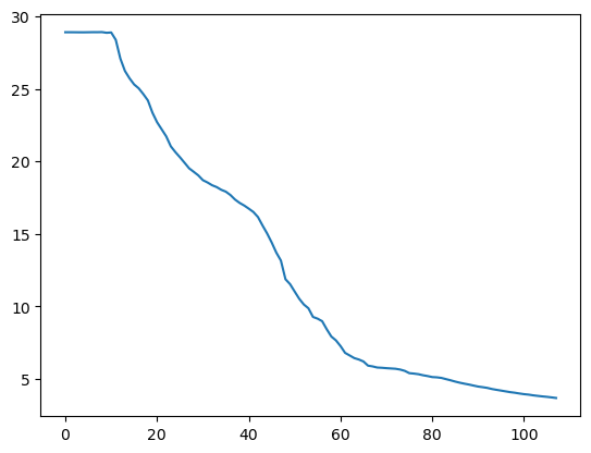
The X axis corresponds to each row in the data and the Y axis is temperature in degrees celcius.

Graphing Salinity Data

---

Now let’s take a look at the pressure and salinity during our Argo float’s dive.

PYTHON

salinity_plot = matplotlib.pyplot.plot(salinity)

Adding Labels to a Graph

It’s good practice to add axes labels to our graphs, these can be done with the xlabel and ylabel functions in matplolib.pyplot.

PYTHON

matplotlib.pyplot.ylabel("Temperature (Degrees C)")
matplotlib.pyplot.xlabel("Reading Number")
temperature_plot = matplotlib.pyplot.plot(temperature)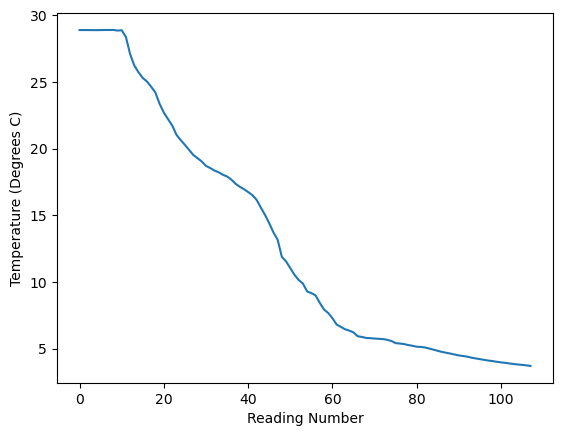

Callout

Importing libraries with shortcuts

So far we use have used the code import matplotlib.pyplot syntax to import the pyplot module of matplotlib. An alternative method for importing is to use import matplotlib.pyplot as plt. Importing pyplot this way means that after the initial import, rather than writing matplotlib.pyplot.plot(...), you can now write plt.plot(...). Another common convention is to use the shortcut import numpy as np when importing the NumPy library. We then can write np.loadtxt(...) instead of numpy.loadtxt(...), for example.

Some people prefer these shortcuts as it is quicker to type and results in shorter lines of code - especially for libraries with long names! You will frequently see Python code online using a pyplot function with plt, or a NumPy function with np, and it’s because they’ve used this shortcut. It makes no difference which approach you choose to take, but you must be consistent as if you use import matplotlib.pyplot as plt then matplotlib.pyplot.plot(...) will not work, and you must use plt.plot(...) instead. Because of this, when working with other people it is important you agree on how libraries are imported. From this point onwards this lesson uses plt to mean matplotlib.pyplot.

Challenge

Plot the pressure data

Create a plot showing the pressure (depth) across a Argo profile.

Show me the solution

PYTHON

import matplotlib.pyplot as plt
plt.xlabel("Reading number")
plt.ylabel("Depth (metres)")
pres_plot = plt.plot(pressure)

Saving Plots

We can call the savefig function to store the plot as a graphics file. This can be a convenient way to store your plots for use in other documents, web pages etc. The graphics format is automatically determined by Matplotlib from the file name ending we specify; here the format is PNG from ‘argo6902746-profile12-temperature.png’. Matplotlib supports many different graphics formats, including SVG, PDF, and JPEG.

PYTHON

matplotlib.pyplot.ylabel("Temperature (Degrees C)")
matplotlib.pyplot.xlabel("Reading Number")
temperature_plot = matplotlib.pyplot.plot(temperature)
matplotlib.pyplot.savefig("argo6902746-profile12-temperature.png")

Plot using Argopy

---

Instead of calling functions in Matplotlib we can also call some plotting functions within Argopy (and these will call Matplotlib for us). This offers two advantages:

1. we don’t need to import matplolib ourselves.
2. there are some Argo specific plots available within Argopy.

Plotting a Map of Where our Float has Travelled

One of the plots that Argopy can generate is a map showing the position of the float every time it surfaced.

PYTHON

float_data = argopy.DataFetcher().float(6902746).load()
argopy.plot.scatter_map(float_data.index, set_global=False)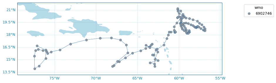

You can also see the same data on an interactive map at https://fleetmonitoring.euro-argo.eu/float/6902746. For some reason the data returned by ArgoPy for this float is limted to the first 118 profiles and there are a few more after that being shown on the fleetmonitoring website.

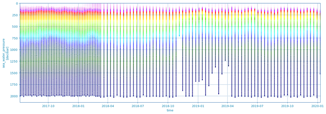
Plotting Temperature Across Multiple Profiles

Another useful feature of the Argopy library is that it can plot data from multiple Argo profiles (dives). This can be done by supplying a whole Xarray dataset for all our profiles; we can extract this from the float_data object we got earlier by calling the to_xarray() function on it. This can be passed to the scatter_plot function in Argopy. We also have to give it the variable name which is “TEMP” (or “PSAL” for salinity). This plot uses colour to show the temperature and puts depth/pressure on the y axis and date on the x axis.

PYTHON

fig = argopy.plot.scatter_plot(float_data.to_xarray(), 'TEMP')

Challenge

Find Another Float to Plot

Pick a different float to load some data from. You can find a list of recently launched UK floats at https://fleetmonitoring.euro-argo.eu/dashboard?Status=Active&Year%20of%20deployment=2025&Country=United%20Kingdom&Network=CORE

Float numbers 7902230, 1902114, 1902725, 1902724, 1902109, 1902111, 1902110, 1902112, 4903834, 4903656, 6990513 or 2903943 could all be good contenders. Some floats will not work because they are missing data and you will ValueError, if this happens try a different float.

Create a new notebook with the following graphs for your float:

• A map showing where it has been
• A scatter plot of temperature against depth over time
• A scatter plot of salinity against depth over time

If you have time add some description about each graph by creating a cell with the Markdown type. Look at https://www.markdownguide.org/basic-syntax/ to see some of the syntax you can use with markdown.

Show me the solution

PYTHON

import argopy
float_data = argopy.DataFetcher().float(7902230).load()
argopy.plot.scatter_map(float_data.index, set_global=False)
fig = argopy.plot.scatter_plot(float_data.to_xarray(), 'TEMP')
fig = argopy.plot.scatter_plot(float_data.to_xarray(), 'PSAL')

Key Points

• “Use the pyplot module from the matplotlib library for creating simple visualisations.”
• “We can give imported modules a short name by using the as keyword after the import.”
• “Argopy has its own built in visaulisation functions”