Content from Python Fundamentals
Last updated on 2026-01-13 | Edit this page
Overview
Questions
- “What basic data types can I work with in Python?”
- “How can I create a new variable in Python?”
- “How do I use a function?”
- “Can I change the value associated with a variable after I create it?”
Objectives
- “Assign values to variables.”
Variables
Any Python interpreter can be used as a calculator:
OUTPUT
23This is great but not very interesting. To do anything useful with
data, we need to assign its value to a variable. In Python, we
can assign a value to a variable, using the equals sign
=. For example, we can track the weight of a patient who
weighs 60 kilograms by assigning the value 60 to a variable
weight_kg:
From now on, whenever we use weight_kg, Python will
substitute the value we assigned to it. In layperson’s terms, a
variable is a name for a value.
In Python, variable names:
- can include letters, digits, and underscores
- cannot start with a digit
- are case sensitive.
This means that, for example: - weight0 is a valid
variable name, whereas 0weight is not - weight
and Weight are different variables
Types of data
Python knows various types of data. Three common ones are:
- integer numbers
- floating point numbers, and
- strings.
In the example above, variable weight_kg has an integer
value of 60. If we want to more precisely track the weight
of our patient, we can use a floating point value by executing:
To create a string, we add single or double quotes around some text. To identify and track a patient throughout our study, we can assign each person a unique identifier by storing it in a string:
Using Variables in Python
Once we have data stored with variable names, we can make use of it in calculations. We may want to store our patient’s weight in pounds as well as kilograms:
We might decide to add a prefix to our patient identifier:
Built-in Python functions
To carry out common tasks with data and variables in Python, the
language provides us with several built-in functions. To display information to
the screen, we use the print function:
OUTPUT
132.66
inflam_001
When we want to make use of a function, referred to as calling the
function, we follow its name by parentheses. The parentheses are
important: if you leave them off, the function doesn’t actually run!
Sometimes you will include values or variables inside the parentheses
for the function to use. In the case of print, we use the
parentheses to tell the function what value we want to display. We will
learn more about how functions work and how to create our own in later
episodes.
We can display multiple things at once using only one
print call:
OUTPUT
inflam_001 weight in kilograms: 60.3We can also call a function inside of another function call. For example,
Python has a built-in function called type that tells you a
value’s data type:
OUTPUT
<class 'float'>
<class 'str'>
Moreover, we can do arithmetic with variables right inside the
print function:
OUTPUT
weight in pounds: 132.66The above command, however, did not change the value of
weight_kg:
OUTPUT
60.3To change the value of the weight_kg variable, we have
to assign weight_kg a new value using the
equals = sign:
OUTPUT
weight in kilograms is now: 75.0Printing variables with f-strings
Earlier on we just printed text in one print statement, and output in a different print statement. However, in the last example, we printed text and output in the same print statement. Python has several ways to achieve this, we can use a comma seperated list of things to print. Another approach is known as “Formatted string literals”, but more commonly called “f-strings”. We need to prefix the string with the letter ‘f’, but then anything within curly brackets is interpreted by python. Variable names can be referenced by wrapping them in ‘{’ and ’} symbols.
F-strings can be used in most cases where we want to print output with text, there are many more advanced options for them that can control things such as the number of decimal places printed out on floating point values.
Variables as Sticky Notes
A variable in Python is analogous to a sticky note with a name written on it: assigning a value to a variable is like putting that sticky note on a particular value.

Using this analogy, we can investigate how assigning a value to one variable does not change values of other, seemingly related, variables. For example, let’s store the subject’s weight in pounds in its own variable:
PYTHON
# There are 2.2 pounds per kilogram
weight_lb = 2.2 * weight_kg
print('weight in kilograms:', weight_kg, 'and in pounds:', weight_lb)
OUTPUT
weight in kilograms: 65.0 and in pounds: 143.0
Similar to above, the expression 2.2 * weight_kg is
evaluated to 143.0, and then this value is assigned to the
variable weight_lb (i.e. the sticky note
weight_lb is placed on 143.0). At this point,
each variable is “stuck” to completely distinct and unrelated
values.
Let’s now change weight_kg:
PYTHON
weight_kg = 100.0
print('weight in kilograms is now:', weight_kg, 'and weight in pounds is still:', weight_lb)
OUTPUT
weight in kilograms is now: 100.0 and weight in pounds is still: 143.0
Since weight_lb doesn’t “remember” where its value comes
from, it is not updated when we change weight_kg.
Comments in Python
Everything in a line of code following the ‘#’ symbol is a comment that is ignored by Python. Comments allow programmers to leave explanatory notes for other programmers or their future selves.
OUTPUT
`mass` holds a value of 47.5, `age` does not exist
`mass` still holds a value of 47.5, `age` holds a value of 122
`mass` now has a value of 95.0, `age`'s value is still 122
`mass` still has a value of 95.0, `age` now holds 102OUTPUT
Hopper Grace- “Basic data types in Python include integers, strings, and floating-point numbers.”
- “Use
variable = valueto assign a value to a variable in order to record it in memory.” - “Variables are created on demand whenever a value is assigned to them.”
- “Use
print(something)to display the value ofsomething.” - “F-strings can be used to display variables without ending quotes
using the syntax
print(f'some text {variable}')” - “Built-in functions are always available to use.”
Content from Analyzing some wave-height data
Last updated on 2026-01-13 | Edit this page
Overview
Questions
- “How can I process tabular data files in Python?”
Objectives
- “Explain what a library is and what libraries are used for.”
- “Import a Python library and use the functions it contains.”
- “Read tabular data from a file into a program.”
- “Select individual values and subsections from data.”
- “Perform operations on arrays of data.”
Words are useful, but what’s more useful are the sentences and stories we build with them. Similarly, while a lot of powerful, general tools are built into Python, specialized tools built up from these basic units live in libraries that can be called upon when needed.
Loading data into Python
To begin processing the wavedata, we need to load it into Python. We can do that using a library called NumPy, which stands for Numerical Python. In general, you should use this library when you want to do fancy things with lots of numbers, especially if you have matrices or arrays. To tell Python that we’d like to start using NumPy, we need to import it:
Importing a library is like getting a piece of lab equipment out of a storage locker and setting it up on the bench. Libraries provide additional functionality to the basic Python package, much like a new piece of equipment adds functionality to a lab space. Just like in the lab, importing too many libraries can sometimes complicate and slow down your programs - so we only import what we need for each program.
Once we’ve imported the library, we can ask the library to read our data file for us:
OUTPUT
array([[1.979e+03, 1.000e+00, 3.788e+00],
       [1.979e+03, 2.000e+00, 3.768e+00],
       [1.979e+03, 3.000e+00, 4.774e+00],
       ...,
       [2.015e+03, 1.000e+01, 3.046e+00],
       [2.015e+03, 1.100e+01, 4.622e+00],
       [2.015e+03, 1.200e+01, 5.048e+00]], shape=(444, 3))
The expression numpy.loadtxt(...) is a function call that asks Python
to run the function
loadtxt which belongs to the numpy library.
The dot notation in Python is used most of all as an object
attribute/property specifier or for invoking its method.
object.property will give you the object.property value,
object_name.method() will invoke on object_name method.
As an example, John Smith is the John that belongs to the Smith
family. We could use the dot notation to write his name
smith.john, just as loadtxt is a function that
belongs to the numpy library.
numpy.loadtxt has two parameters: the name of the file we
want to read and the delimiter
that separates values on a line. These both need to be character strings
(or strings for short), so we put
them in quotes. Notice that we also had to tell NumPy to skip the first
row, which contains the column titles.
Since we haven’t told it to do anything else with the function’s
output, the notebook displays it.
In this case, that output is the data we just loaded. By default, only a
few rows and columns are shown (with ... to omit elements
when displaying big arrays). Note that, to save space when displaying
NumPy arrays, Python does not show us trailing zeros, so
1.0 becomes 1..
Our call to numpy.loadtxt read our file but didn’t save
the data in memory. To do that, we need to assign the array to a
variable. In a similar manner to how we assign a single value to a
variable, we can also assign an array of values to a variable using the
same syntax. Let’s re-run numpy.loadtxt and save the
returned data:
This statement doesn’t produce any output because we’ve assigned the
output to the variable data. If we want to check that the
data have been loaded, we can print the variable’s value:
OUTPUT
[[1.979e+03 1.000e+00 3.788e+00]
 [1.979e+03 2.000e+00 3.768e+00]
 [1.979e+03 3.000e+00 4.774e+00]
 ...
 [2.015e+03 1.000e+01 3.046e+00]
 [2.015e+03 1.100e+01 4.622e+00]
 [2.015e+03 1.200e+01 5.048e+00]]
Now that the data are in memory, we can manipulate them. First, let’s
ask what type of thing
data refers to:
OUTPUT
<class 'numpy.ndarray'>The output tells us that data currently refers to an
N-dimensional array, the functionality for which is provided by the
NumPy library. These data correspond to sea wave height. Each row is a
monthly average, and the columns are their associated dates and
values.
Data Type
A Numpy array contains one or more elements of the same type. The
type function will only tell you that a variable is a NumPy
array but won’t tell you the type of thing inside the array. We can find
out the type of the data contained in the NumPy array.
OUTPUT
float64This tells us that the NumPy array’s elements are floating-point numbers.
With the following command, we can see the array’s shape:
OUTPUT
(444, 3)The output tells us that the data array variable
contains 444 rows (sanity check: 37 years of 12 months = 37 * 12 = 444)
and 3 columns (year, month, and datapoint). When we created the variable
data to store our wave data, we did not only create the
array; we also created information about the array, called members or attributes. This extra
information describes data in the same way an adjective
describes a noun. data.shape is an attribute of
data which describes the dimensions of data.
We use the same dotted notation for the attributes of variables that we
use for the functions in libraries because they have the same
part-and-whole relationship.
If we want to get a single number from the array, we must provide an index in square brackets after the variable name, just as we do in math when referring to an element of a matrix. Our wave data has two dimensions, so we will need to use two indices to refer to one specific value:
OUTPUT
first value in data: 3.788OUTPUT
middle value in data: 2.446The expression data[222, 2] accesses the element on the
223rd row and 3rd column. While this expression may not surprise you,
using data[0, 2] to get the 3rd column in the
1st row might. Programming languages like Fortran, MATLAB and R
start counting at 1 because that’s what human beings have done for
thousands of years. Languages in the C family (including C++, Java,
Perl, and Python) count from 0 because it represents an offset from the
first value in the array (the second value is offset by one index from
the first value). This is closer to the way that computers represent
arrays (if you are interested in the historical reasons behind counting
indices from zero, you can read Mike
Hoye’s blog post). As a result, if we have an M×N array in Python,
its indices go from 0 to M-1 on the first axis and 0 to N-1 on the
second. It takes a bit of getting used to, but one way to remember the
rule is that the index is how many steps we have to take from the start
to get the item we want.
!['data' is a 3 by 3 numpy array containing row 0: ['A', 'B', 'C'], row 1: ['D', 'E', 'F'], and row 2: ['G', 'H', 'I']. Starting in the upper left hand corner, data[0, 0] = 'A', data[0, 1] = 'B', data[0, 2] = 'C', data[1, 0] = 'D', data[1, 1] = 'E', data[1, 2] = 'F', data[2, 0] = 'G', data[2, 1] = 'H', and data[2, 2] = 'I', in the bottom right hand corner.](fig/python-zero-index.svg)
In the Corner
What may also surprise you is that when Python displays an array, it
shows the element with index [0, 0] in the upper left
corner rather than the lower left. This is consistent with the way
mathematicians draw matrices but different from the Cartesian
coordinates. The indices are (row, column) instead of (column, row) for
the same reason, which can be confusing when plotting data.
Slicing data
An index like [222, 2] selects a single element of an
array, but we can select whole sections as well. For example, we can
select the wavedata for the first year like this:
OUTPUT
[[1.979e+03 1.000e+00 3.788e+00]
 [1.979e+03 2.000e+00 3.768e+00]
 [1.979e+03 3.000e+00 4.774e+00]
 [1.979e+03 4.000e+00 2.818e+00]
 [1.979e+03 5.000e+00 2.734e+00]
 [1.979e+03 6.000e+00 2.086e+00]
 [1.979e+03 7.000e+00 2.066e+00]
 [1.979e+03 8.000e+00 2.236e+00]
 [1.979e+03 9.000e+00 3.322e+00]
 [1.979e+03 1.000e+01 3.512e+00]
 [1.979e+03 1.100e+01 4.348e+00]
 [1.979e+03 1.200e+01 4.628e+00]]
The slice 0:12 means,
“Start at index 0 and go up to, but not including, index 12”. Again, the
up-to-but-not-including takes a bit of getting used to, but the rule is
that the difference between the upper and lower bounds is the number of
values in the slice.
We don’t have to start slices at 0:
OUTPUT
[[ 1.     3.666]
 [ 2.     4.326]
 [ 3.     3.522]
 [ 4.     3.18 ]
 [ 5.     1.954]
 [ 6.     1.72 ]
 [ 7.     1.86 ]
 [ 8.     1.95 ]
 [ 9.     3.11 ]
 [10.     3.78 ]
 [11.     3.474]
 [12.     5.28 ]]
We also don’t have to include the upper and lower bound on the slice. If we don’t include the lower bound, Python uses 0 by default; if we don’t include the upper, the slice runs to the end of the axis, and if we don’t include either (i.e., if we use ‘:’ on its own), the slice includes everything:
The above example selects rows 0 through 11 and columns 2 through to the end of the array (which in this case is only the last column).
OUTPUT
data from first year is:
[[3.788]
 [3.768]
 [4.774]
 [2.818]
 [2.734]
 [2.086]
 [2.066]
 [2.236]
 [3.322]
 [3.512]
 [4.348]
[4.628]]Slicing Strings
A section of an array is called a slice. We can take slices of character strings as well:
PYTHON
element = 'oxygen'
print('first three characters:', element[0:3])
print('last three characters:', element[3:6])
OUTPUT
first three characters: oxy
last three characters: gen
What is the value of element[:4]? What about
element[4:]? Or element[:]?
OUTPUT
oxyg
en
oxygenSlicing Strings (continued)
What is element[-1]? What is
element[-2]?
OUTPUT
n
eSlicing Strings (continued)
Given those answers, explain what element[1:-1]
does.
Creates a substring from index 1 up to (not including) the final index, effectively removing the first and last letters from ‘oxygen’
Slicing Strings (continued)
How can we rewrite the slice for getting the last three characters of
element, so that it works even if we assign a different
string to element? Test your solution with the following
strings: carpentry, clone,
hi.
PYTHON
element = 'oxygen'
print('last three characters:', element[-3:])
element = 'carpentry'
print('last three characters:', element[-3:])
element = 'clone'
print('last three characters:', element[-3:])
element = 'hi'
print('last three characters:', element[-3:])
OUTPUT
last three characters: gen
last three characters: try
last three characters: one
last three characters: hiThin Slices
The expression element[3:3] produces an empty string, i.e., a string that
contains no characters. If data holds our array of wave
data, what does data[3:3, 4:4] produce? What about
data[3:3, :]?
Analyzing data
NumPy has several useful functions that take an array as input to
perform operations on its values. If we want to find the average wave
height for all months on all years, for example, we can ask NumPy to
compute data’s mean value:
OUTPUT
668.9611876876877mean is a function
that takes an array as an argument. Given that our array
contains the dates as well as data, with numbers relating to years and
months, taking the mean of the whole array doesn’t really make much
sense - we don’t expect to see 600 metre high waves!
We can use slicing to calculate the correct mean:
OUTPUT
3.383563063063063Not All Functions Have Input
Generally, a function uses inputs to produce outputs. However, some functions produce outputs without needing any input. For example, checking the current time doesn’t require any input.
OUTPUT
Sat Mar 26 13:07:33 2016For functions that don’t take in any arguments, we still need
parentheses (()) to tell Python to go and do something for
us.
Let’s use three other NumPy functions to get some descriptive values about the wave heights. We’ll also use multiple assignment, a convenient Python feature that will enable us to do this all in one line.
PYTHON
maxval, minval, stdval = numpy.max(data[:,2]), numpy.min(data[:,2]), numpy.std(data[:,2])

print('Max wave height:', maxval)
print('Min wave height:', minval)
print('Wave height standard deviation:', stdval)
Here we’ve assigned the return value from
numpy.max(data[:,2]) to the variable maxval,
the value from numpy.min(data[:,2]) to minval,
and so on. Note that we used maxval, rather than just
max - it’s not good practice to use variable names that are
the same as Python
keywords or fuction names.
OUTPUT
Max wave height: 6.956
Min wave height: 1.496
Wave height standard deviation: 1.1440155050316319Getting help on functions
How did we know what functions NumPy has and how to use them? If you
are working in IPython or in a Jupyter Notebook, there is an easy way to
find out. If you type the name of something followed by a dot, then you
can use tab completion
(e.g. type numpy. and then press Tab) to see a
list of all functions and attributes that you can use. After selecting
one, you can also add a question mark
(e.g. numpy.cumprod?), and IPython will return an
explanation of the method! This is the same as doing
help(numpy.cumprod). Similarly, if you are using the “plain
vanilla” Python interpreter, you can type numpy. and press
the Tab key twice for a listing of what is available. You can
then use the help() function to see an explanation of the
function you’re interested in, for example:
help(numpy.cumprod).
What about NaNs?
In real datasets, particularly ones which come from observational data, it’s quite common for some values to be missing. There are various strategies to deal with missing values; one of which is to give them a value that would be clearly wrong (e.g. -1 for a temperature column with units in Kelvin, or 999 for a missing latitude or longitude value). However, the issue with this is that we would need to check for these values before calculating any summary statistic.
Instead, we can use NumPy’s nan (“not a number”) value,
which will tell NumPy that these are values that need to be dealt with
in a special manner. NumPy also provides various functions to help deal
with NaNs.
Beware the NumPy version 1.x used NaN and numpy version
2.x uses nan, this course assumes you have Numpy version
2.x installed and will use that convention.
However, we can’t use NumPy’s normal statistical functions on any array that contains a NaN, as this returns a NaN:
Instead, we need to use the NumPy function nanmean:
If, at a later date, we’d like to replace all the NaNs with a sensible numerical value (e.g. the mean of the column), NumPy also provides functions that can help with this
What happens if the shape of the data is not convenient for
us to do some of our analysis? With this waveheight dataset, the data is
a time-series, but it’s not very easy to calculate things like average
monthly temperature. To do that, we’ll need to reshape it.
Numpy allows us to do that relatively easily:
PYTHON
reshaped_data = numpy.reshape(data[:,2], [37,12]) # reshape the data to form a 2D array of year by monthWe now have a 2D array of data using, where each row is a year, and each column represents a month:
OUTPUT
The shape of the reshaped data is:
(37, 12)
We can verify that nothing about the data has changed:
PYTHON
print(f"The maximum value of the reshaped data is: {numpy.max(reshaped_data)}")
print(f"The minimum value of the reshaped data is: {numpy.min(reshaped_data)}")
print(f"The standard deviation of the reshaped data is: {numpy.std(reshaped_data)}")
OUTPUT
The maximum value of the reshaped data is: 6.956
The minimum value of the reshaped data is: 1.496
The standard deviation of the reshaped data is: 1.1440155050316319
We can now look variations in some summary statistics, such as the maximum wave height per month, or average height per year more easily. One way to do this is to create a new temporary array of the data we want, then ask it to do the calculation:
PYTHON
year_0 = reshaped_data[0,:] # 0 on the first axis (rows), everything on the second (columns)
print(f"maximum wave height for year 0: {numpy.max(year_0)}")
OUTPUT
maximum wave height for year 0: 4.774What if we need the maximum wave height for each month over all years (as in the next diagram on the left) or the average for each month (as in the diagram on the right)? As the diagram below shows, we want to perform the operation across an axis:
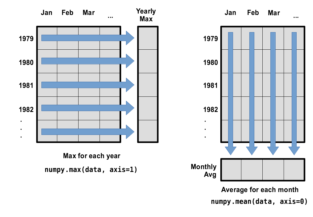
To support this functionality, most array functions allow us to specify the axis we want to work on. If we ask for the average across axis 0 (rows in our 2D example), we get:
OUTPUT
[4.59956757 4.39708108 4.09156757 3.26016216 2.60437838 2.3072973
 2.18940541 2.32145946 2.9907027  3.55627027 3.90345946 4.38140541]
As a quick check, we can ask this array what its shape is:
OUTPUT
(12,)The expression (12,) tells us we have an N×1 vector, so
this is the average wave height per month for all years. If we average
across axis 1 (columns in our 2D example), we get:
OUTPUT
[3.34       3.15183333 3.29866667 3.53366667 3.448      3.23016667
 2.99383333 3.51133333 2.96066667 3.20316667 3.62116667 5.1915
 3.28816667 3.529      3.523      3.66866667 3.314      2.99916667
 3.45983333 3.16783333 3.413      3.3435     3.031      3.29366667
 3.138      3.29716667 3.3185     3.24966667 3.4135     3.42866667
 3.168      2.78816667 3.61366667 3.2725     3.32766667 3.2765
 4.385     ]
which is the average wave height per year across all months.
Saving Data
There are occasions though the rest of the lesson when we will want to use the reshaped data. If we close this Notebook, we’ll lose the variables we’ve created, so let’s save the reshaped data to a file:
Stacking Arrays
Arrays can be concatenated and stacked on top of one another, using
NumPy’s vstack and hstack functions for
vertical and horizontal stacking, respectively.
PYTHON
A = numpy.array([[1,2,3], [4,5,6], [7, 8, 9]])
print('A = ')
print(A)
>
B = numpy.hstack([A, A])
print('B = ')
print(B)
>
C = numpy.vstack([A, A])
print('C = ')
print(C)
OUTPUT
A =
[[1 2 3]
 [4 5 6]
 [7 8 9]]
B =
[[1 2 3 1 2 3]
 [4 5 6 4 5 6]
 [7 8 9 7 8 9]]
C =
[[1 2 3]
 [4 5 6]
 [7 8 9]
 [1 2 3]
 [4 5 6]
 [7 8 9]]
Write some additional code that slices the first and last columns of
A, and stacks them into a 3x2 array. Make sure to
print the results to verify your solution.
A ‘gotcha’ with array indexing is that singleton dimensions are
dropped by default. That means A[:, 0] is a one dimensional
array, which won’t stack as desired. To preserve singleton dimensions,
the index itself can be a slice or array. For example,
A[:, :1] returns a two dimensional array with one singleton
dimension (i.e. a column vector).
OUTPUT
D =
[[1 3]
 [4 6]
[7 9]]Change In Wave Height
In the wave data, one row represents a series of monthly data relating to one year. This means that the change in height over time is a meaningful concept representing seasonal changes. Let’s find out how to calculate changes in the data contained in an array with NumPy.
The numpy.diff() function takes an array and returns the
differences between two successive values. Let’s use it to examine the
changes each day across the first 6 months of waves in year 4 from our
dataset.
OUTPUT
[3.73 4.886 4.76 3.188 2.528 1.662 1.952 2.388 3.336 4.034 4.502 5.438]Calling numpy.diff(year4) would do the following
calculations
OUTPUT
[ 4.886 - 3.73, 4.76 - 4.886, 3.188 - 4.76, 2.528 - 3.188, 1.662 - 2.528, 1.952 - 1.662, 2.388 - 1.952, 3.336 - 2.388, 4.034 - 3.336, 4.502 - 4.034, 5.438 - 4.502 ]and return the 11 difference values in a new array.
OUTPUT
[ 1.156 -0.126 -1.572 -0.66  -0.866  0.29   0.436  0.948  0.698  0.468
 0.936]
Note that the array of differences is shorter by one element (length 11). Where we see a negative change in wave height, it shows that the sea is becoming calmer as we move towards the summer. Positive wave heights in the autumn show waves are increasing.
If the shape of an individual data file is (60, 40) (60
rows and 40 columns), what would the shape of the array be after you run
the diff() function and why?
The shape will be (60, 39) because there is one fewer
difference between columns than there are columns in the data. {:
.solution}
How would you find the largest change in wave height from month to month within each year? What does it mean if the change in height is an increase or a decrease?
By using the numpy.max() function after you apply the
numpy.diff() function, you will get the largest difference
between months.
OUTPUT
array([1.086, 1.806, 1.776, 1.156, 1.692, 1.274, 0.798, 2.59 , 1.338,
      1.634, 0.992, 0.618, 1.054, 1.652, 1.472, 1.716, 0.766, 1.496,
      1.656, 1.04 , 1.228, 1.336, 1.564, 1.066, 1.242, 1.604, 0.802,
      1.04 , 0.652, 0.86 , 1.176, 0.97 , 1.68 , 1.556, 1.904, 2.936,
      1.578])
If wave height values decrease along an axis, then the
difference from one element to the next will be negative. If you are
interested in the magnitude of the change and not the
direction, the numpy.absolute() function will provide
that.
Notice the difference if you get the largest absolute difference between readings.
OUTPUT
array([1.956, 1.806, 1.776, 1.572, 3.6  , 2.418, 0.954, 2.798, 1.338,
       1.634, 2.13 , 0.93 , 1.054, 1.71 , 1.68 , 2.   , 1.614, 1.496,
       2.308, 1.04 , 2.014, 1.68 , 1.564, 1.596, 1.528, 1.604, 1.468,
       1.21 , 1.012, 0.86 , 1.732, 1.03 , 1.68 , 1.774, 1.904, 2.936,
1.694])- “Import a library into a program using
import libraryname.” - “Use the
numpylibrary to work with arrays in Python.” - “The expression
array.shapegives the shape of an array.” - “Use
array[x, y]to select a single element from a 2D array.” - “Array indices start at 0, not 1.”
- “Use
low:highto specify aslicethat includes the indices fromlowtohigh-1.” - “Use
# some kind of explanationto add comments to programs.” - “Use
numpy.mean(array),numpy.max(array), andnumpy.min(array)to calculate simple statistics.” - “Use
numpy.mean(array, axis=0)ornumpy.mean(array, axis=1)to calculate statistics across the specified axis.”
Content from Visualizing Tabular Data
Last updated on 2026-01-13 | Edit this page
Overview
Questions
- “How can I visualize tabular data in Python?”
- “How can I group several plots together?”
Objectives
- “Plot simple graphs from data.”
- “Plot multiple graphs in a single figure.”
Visualizing data
The mathematician Richard Hamming once said, “The purpose of
computing is insight, not numbers,” and the best way to develop insight
is often to visualize data. Visualization deserves an entire lecture of
its own, but we can explore a few features of Python’s
matplotlib library here. While there is no official
plotting library, matplotlib is the de facto
standard. First, we will import the pyplot module from
matplotlib and use two of its functions to create and
display a heat map of our
data:
Episode Prerequisites
If you are continuing in the same notebook from the previous episode,
you already have a reshaped_data variable and have imported
numpy.
For ease, let’s rename the variable:
If you are starting a new notebook at this point, you need the following three lines:
PYTHON
import numpy
data = numpy.loadtxt(fname='wavesmonthly.csv', delimiter=',', skiprows=1)
data = numpy.reshape(data[:,2], [37,12])
…or, if you saved the reshaped data into a file
Now let’s use the Matplotlib library to plot this data. We’ll need to
import from the matplotlib.pyplot library. We can then use
the imshow function to plot this data. In some versions of
Python we’ll need to call the show function to display the
graph. This will plot a heatmap of our data.
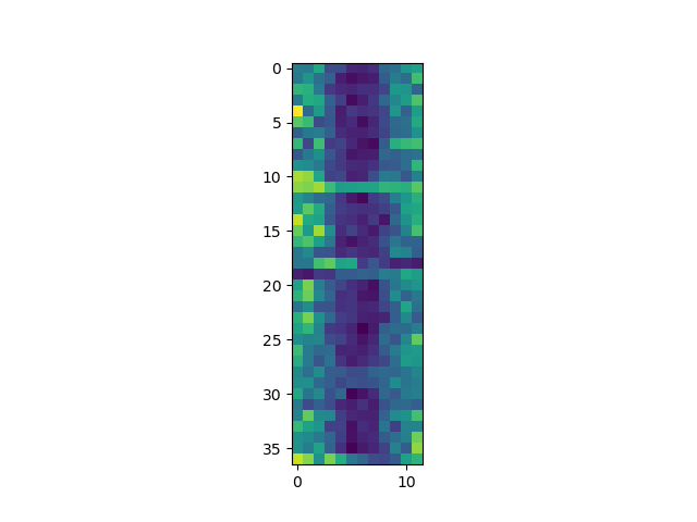
Each row in the heat map corresponds to a year in the dataset, and each column corresponds to a month. Blue pixels in this heat map represent low values, while yellow pixels represent high values. We can see low blue values in the middle (summer) months, and higher waves at the start and end of the year. This demonstrates that there is a seasonal cycle present. With calm summers bringing lower waves, and windy winters generating big waves. There are still differences year to year, with some stormier summers and calmer winters.
Now let’s take a look at the average wave-height per month over time.
Here we’ll used the plot function to plot a line graph.
PYTHON
ave_waveheight = numpy.mean(data, axis=0)
ave_plot = matplotlib.pyplot.plot(ave_waveheight)
matplotlib.pyplot.show()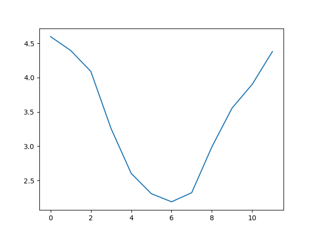
This is a good way to smooth out variability, and see what is called a ‘climatology’, representing the long-term wave climate over several years or decades.
Here, we have put the average wave heights per month across all years
in the array ave_waveheight, then asked
matplotlib.pyplot to create and display a line graph of
those values. The result is a smooth seasonal cycle, with a maximum in
month 0 (January) and minimum in month 6 (July). But a good data
scientist doesn’t just consider the average of a dataset, so let’s have
a look at the minimum and maximum too. It’s good practice to add axes
labels to our graphs, these can be done with the xlabel and
ylabel functions in matplolib.pyplot.
PYTHON
matplotlib.pyplot.ylabel("Max Wave Height (metres)")
matplotlib.pyplot.xlabel("Month")
max_plot = matplotlib.pyplot.plot(numpy.max(data, axis=0))
matplotlib.pyplot.show()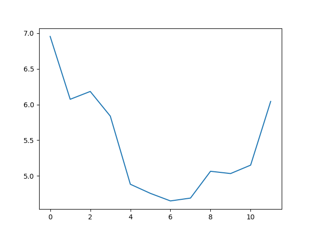
PYTHON
matplotlib.pyplot.ylabel("Min Wave Height (metres)")
matplotlib.pyplot.xlabel("Month")
min_plot = matplotlib.pyplot.plot(numpy.min(data, axis=0))
matplotlib.pyplot.show()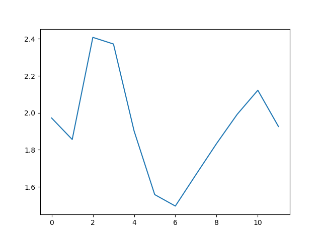
The minimum and maximum graphs show the large spread of all possible wave heights throughout the dataset. There is still a seasonal cycle, but less clear as the extremes are much less smooth. The maximum wave heights can reach a massive 7 metres, and even in the summer the maximum is 4.5m (around the height of a double decker bus!) The minimum values are more similar throughout the year, varying between 1.5 and 2.5 metres.
Plotting the data in this way, allows us to get a broad picture of the wave climate, without having to examine the numbers themselves without visualization tools.
Grouping plots
You can group similar plots in a single figure using subplots. This
script below uses a number of new commands. The function
matplotlib.pyplot.figure() creates a space into which we
will place all of our plots. The parameter figsize tells
Python how big to make this space. Each subplot is placed into the
figure using its add_subplot method. The add_subplot
method takes 3 parameters. The first denotes how many total rows of
subplots there are, the second parameter refers to the total number of
subplot columns, and the final parameter denotes which subplot your
variable is referencing (left-to-right, top-to-bottom). Each subplot is
stored in a different variable (axes1, axes2,
axes3). Once a subplot is created, the axes can be titled
using the set_xlabel() command (or
set_ylabel()), note these are different to the
xlabel and ylabel functions used by
matplot.pyplot. Let’s create three new plots, side by side,
this time showing within each of the 37 years of the dataset - notice
how we now use axis=1 in our calls to the summary statistic
functions:
PYTHON
fig = matplotlib.pyplot.figure(figsize=(10.0, 3.0))

axes1 = fig.add_subplot(1, 3, 1)
axes2 = fig.add_subplot(1, 3, 2)
axes3 = fig.add_subplot(1, 3, 3)

axes1.set_ylabel('Average')
axes1.set_xlabel('Year index')
axes1.plot(numpy.mean(data, axis=1))

axes2.set_ylabel('Max')
axes2.set_xlabel('Year index')
axes2.plot(numpy.max(data, axis=1))

axes3.set_ylabel('Min')
axes3.set_xlabel('Year index')
axes3.plot(numpy.min(data, axis=1))

fig.tight_layout()

matplotlib.pyplot.savefig('wavedata.png')
matplotlib.pyplot.show()
This script tells the plotting library how large we want the figure
to be, that we’re creating three subplots, what to draw for each one,
and that we want a tight layout. (If we leave out that call to
fig.tight_layout(), the graphs will actually be squeezed
together more closely.)
The call to savefig stores the plot as a graphics file.
This can be a convenient way to store your plots for use in other
documents, web pages etc. The graphics format is automatically
determined by Matplotlib from the file name ending we specify; here PNG
from ‘wavedata.png’. Matplotlib supports many different graphics
formats, including SVG, PDF, and JPEG.
Importing libraries with shortcuts
So far we use have used the code
import matplotlib.pyplot syntax to import the
pyplot module of matplotlib. An alternative
method for importing is to use
import matplotlib.pyplot as plt. Importing
pyplot this way means that after the initial import, rather
than writing matplotlib.pyplot.plot(...), you can now write
plt.plot(...). Another common convention is to use the
shortcut import numpy as np when importing the NumPy
library. We then can write np.loadtxt(...) instead of
numpy.loadtxt(...), for example.
Some people prefer these shortcuts as it is quicker to type and
results in shorter lines of code - especially for libraries with long
names! You will frequently see Python code online using a
pyplot function with plt, or a NumPy function
with np, and it’s because they’ve used this shortcut. It
makes no difference which approach you choose to take, but you must be
consistent as if you use import matplotlib.pyplot as plt
then matplotlib.pyplot.plot(...) will not work, and you
must use plt.plot(...) instead. Because of this, when
working with other people it is important you agree on how libraries are
imported. From this point onwards this lesson uses plt to
mean matplotlib.pyplot.
Plot Scaling
Why do all of our plots stop just short of the upper end of our graph?
Because matplotlib normally sets x and y axes limits to the min and max of our data (depending on data range)
Plotting multiple graphs on one pair of axes
We can also plot more than one dataset on a single pair of axes, and Matplotlib gives us lots of control over the output. Can you plot the maximum, minimum, and mean all on the same axes, change the colour and marker used for each of the plots, and give the plot a legend?
We can call plot multiple times before we call
show, and each of those will be added to the axes. We can
also specify format options as a string (this needs to specified
straight after the data to plot), with all available options listed in
the
documentation. We also need to specify the label for
each plot, and call legend() to make the legend
visible.
An example would be
PYTHON
import matplotlib.pyplot as plt
plt.plot(numpy.max(data, axis=0), "bo", label='Maximum')
plt.plot(numpy.average(data, axis=0), "m+", label='Average')
plt.plot(numpy.min(data, axis=0), "r--", label='Minumum')
plt.legend(loc='best')

plt.show()
Make Your Own Plot
Create a plot showing the standard deviation (numpy.std)
of the wave data across all months.
Moving Plots Around
Modify the program to display the three plots on top of one another instead of side by side.
PYTHON
# change figsize (swap width and height)
fig = plt.figure(figsize=(3.0, 10.0))

# change add_subplot (swap first two parameters)
axes1 = fig.add_subplot(3, 1, 1)
axes2 = fig.add_subplot(3, 1, 2)
axes3 = fig.add_subplot(3, 1, 3)

axes1.set_ylabel('average')
axes1.plot(numpy.mean(data, axis=1))

axes2.set_ylabel('max')
axes2.plot(numpy.max(data, axis=1))

axes3.set_ylabel('min')
axes3.plot(numpy.min(data, axis=1))

fig.tight_layout()

plt.show()
NetCDF files
What about data stored in other types of files? Scientific data is often stored in NetCDF files. We can also read these files easily with python, but we use to use a different library
We will again use data describing sea waves, but this time looking at a spatial map. This data set shows a static world map, containing data with the multi-year average wave climate. Again, hs_avg is the wave height in metres. But this time, the shape of the matrix is latitude x longitude
Using other libraries
For the rest of this lesson, we need to use a python library that isn’t included in the default installation of Anaconda. There are various ways to doing this, depending on how you opened the Jupyter Notebook:
If you’re using Anaconda Navigator: - return to the main window of
Anaconda Navigator - select “Environments” from the left-hand menu, and
then “base (root)” - Select the Not Installed filter
option to list all packages that are available in the environment’s
channels, but not installed. - Select the name of the package you want
to install. We want NetCDF4 - Click Apply
If you opened the Jupyter Notebook via the command line: - you’ll
need to close the Notebook (Ctrl+C, twice) - run the command
conda install netcdf4, and accept any prompt(s)
(y)
We can then import a netCDF file, and check to see what python thinks its type is:
OUTPUT
<class 'netCDF4._netCDF4.Dataset'>We can use Matplotlib to display this data set as a world map. The data go from -90 degrees (south pole) to +90 degrees (north pole) in the y direction. In the x-direction the data go from 0 to 360 degrees East, starting at the Greenwich meridian. The white areas are land, because we have no data there to plot.
PYTHON
plt.xlabel("Longitude")
plt.ylabel("Latitude")
plt.imshow(globaldata["hs_avg"][0], extent=[0,360,-90,90], origin='lower')
plt.show()
NetCDF files can be quite complex, and normally consist of a number
of variables stored as 2D or 3D arrays.
globaldata["hs_avg"] is getting a variable called
hs_avg (average significant wave height), which is of type
netCDF4._netCDF4.Variable (the full list of variables
stored can be listed with globaldata.variables.keys()). We
can use the first element of globaldata["hs_avg"] to plot
the global map using the imshow() function. Although the
type of this element is numpy.ma.core.MaskedArray, the
imshow() function can natively use this variable type as
input.
We then need to specify that the data axes of the plot need to go
from 0 to 360 on the x-axis, and -90 to 90 on the y-axis. We also use
origin='lower' to stop the map being displayed upside down,
because we want the map being plotted from the bottom-left, rather than
the top-left which is the default for plotting matrix-type data (because
this is where [0:0] normally is).
We can also add a colour bar to help describe the figure, with a little more code:
PYTHON
fig = plt.figure(figsize=(12.0,4.0))
ax = plt.gca()
ax.set_xlabel("Longitude")
ax.set_ylabel("Latitude")
im = ax.imshow(globaldata["hs_avg"][0], extent=[0,360,-90,90], origin='lower')
cbar = fig.colorbar(im, ax=ax, location="right", pad=0.02)
plt.show()
Investigate NetCDF Metadata
NetCDF files don’t just include data, they also include metadata
describing their data. If we print the globaldata object we
can see some of this data.
Print the dataset and find out the following:
- When was this dataset created?
- How many timesteps are there in the data?
- What date range does the data cover?
Accessing subsets of NetCDF data
How might we get the value of first timestep at the Northernmost and Westernmost point?
How could we access a North/South transect through the data at the 180th longitude point and first timestep? Make a graph of this data.
- “Use the
pyplotmodule from thematplotliblibrary for creating simple visualizations.”
Content from Storing Multiple Values in Lists
Last updated on 2026-01-14 | Edit this page
Overview
Questions
- “How can I store many values together?”
Objectives
- “Explain what a list is.”
- “Create and index lists of simple values.”
- “Change the values of individual elements”
- “Append values to an existing list”
- “Reorder and slice list elements”
- “Create and manipulate nested lists”
In the previous episode, we analyzed a single file of wave height data. However we might need to process multiple files in future.
There are four decadal CSV files for the 1980s, 1990s, 2000s, and 2010s. Before we can analyse these, we need to learn how to store an arbitary number of items in a list.
The natural first step is to collect the names of all the files that we have to process. In Python, a list is a way to store multiple values together. In this episode, we will learn how to store multiple values in a list as well as how to work with lists.
Python lists
Unlike NumPy arrays, lists are built into the language so we do not have to load a library to use them. We create a list by putting values inside square brackets and separating the values with commas:
OUTPUT
odds are: [1, 3, 5, 7]We can access elements of a list using indices – numbered positions of elements in the list. These positions are numbered starting at 0, so the first element has an index of 0.
PYTHON
print('first element:', odds[0])
print('last element:', odds[3])
print('"-1" element:', odds[-1])
OUTPUT
first element: 1
last element: 7
"-1" element: 7
Yes, we can use negative numbers as indices in Python. When we do so,
the index -1 gives us the last element in the list,
-2 the second to last, and so on. Because of this,
odds[3] and odds[-1] point to the same element
here.
There is one important difference between lists and strings: we can change the values in a list, but we cannot change individual characters in a string. For example:
PYTHON
names = ['Curie', 'Darwing', 'Turing']  # typo in Darwin's name
print('names is originally:', names)
names[1] = 'Darwin'  # correct the name
print('final value of names:', names)
OUTPUT
names is originally: ['Curie', 'Darwing', 'Turing']
final value of names: ['Curie', 'Darwin', 'Turing']
works, but:
OUTPUT
---------------------------------------------------------------------------
TypeError                                 Traceback (most recent call last)
<ipython-input-8-220df48aeb2ein <module>()
      1 name = 'Darwin'
----2 name[0] = 'd'

TypeError: 'str' object does not support item assignment
does not.
Ch-Ch-Ch-Ch-Changes
Data which can be modified in place is called mutable, while data which cannot be modified is called immutable. Strings and numbers are immutable. This does not mean that variables with string or number values are constants, but when we want to change the value of a string or number variable, we can only replace the old value with a completely new value.
Lists and arrays, on the other hand, are mutable: we can modify them after they have been created. We can change individual elements, append new elements, or reorder the whole list. For some operations, like sorting, we can choose whether to use a function that modifies the data in-place or a function that returns a modified copy and leaves the original unchanged.
Be careful when modifying data in-place. If two variables refer to the same list, and you modify the list value, it will change for both variables!
PYTHON
salsa = ['peppers', 'onions', 'cilantro', 'tomatoes']
my_salsa = salsa        # <-- my_salsa and salsa point to the *same* list data in memory
salsa[0] = 'hot peppers'
print('Ingredients in my salsa:', my_salsa)
OUTPUT
Ingredients in my salsa: ['hot peppers', 'onions', 'cilantro', 'tomatoes']If you want variables with mutable values to be independent, you must make a copy of the value when you assign it.
PYTHON
salsa = ['peppers', 'onions', 'cilantro', 'tomatoes']
my_salsa = list(salsa)        # <-- makes a *copy* of the list
salsa[0] = 'hot peppers'
print('Ingredients in my salsa:', my_salsa)
OUTPUT
Ingredients in my salsa: ['peppers', 'onions', 'cilantro', 'tomatoes']Because of pitfalls like this, code which modifies data in place can be more difficult to understand. However, it is often far more efficient to modify a large data structure in place than to create a modified copy for every small change. You should consider both of these aspects when writing your code.
Nested Lists
Since a list can contain any Python variables, it can even contain other lists.
For example, you could represent the products on the shelves of a
small grocery shop as a nested list called veg:
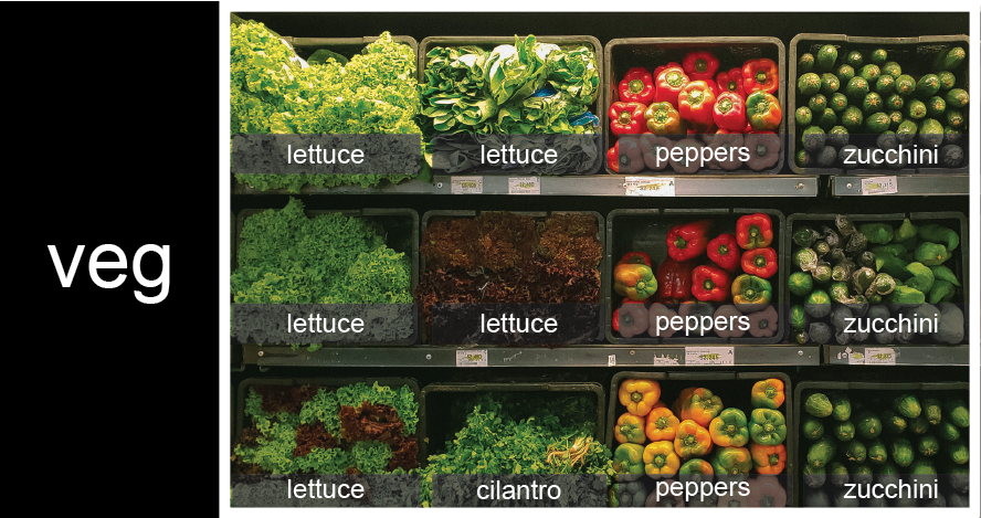
To store the contents of the shelf in a nested list, you write it this way:
PYTHON
veg = [['lettuce', 'lettuce', 'peppers', 'zucchini'],
     ['lettuce', 'lettuce', 'peppers', 'zucchini'],
     ['lettuce', 'cilantro', 'peppers', 'zucchini']]
Here are some visual examples of how indexing a list of lists
veg works. First, you can reference each row on the shelf
as a separate list. For example, veg[2] represents the
bottom row, which is a list of the baskets in that row.
![veg is now shown as a list of three rows, with veg[0] representing the top row of three baskets, veg[1] representing the second row, and veg[2] representing the bottom row.](fig/04_groceries_veg0.png)
Index operations using the image would work like this:
OUTPUT
['lettuce', 'cilantro', 'peppers', 'zucchini']OUTPUT
['lettuce', 'lettuce', 'peppers', 'zucchini']To reference a specific basket on a specific shelf, you use two
indexes. The first index represents the row (from top to bottom) and the
second index represents the specific basket (from left to right). ![veg is now shown as a two-dimensional grid, with each basket labeled according to its index in the nested list. The first index is the row number and the second index is the basket number, so veg[1][3] represents the basket on the far right side of the second row (basket 4 on row 2): zucchini](fig/04_groceries_veg00.png)
OUTPUT
'lettuce'OUTPUT
'peppers'Heterogeneous Lists
Lists in Python can contain elements of different types. Example:
There are many ways to change the contents of lists besides assigning new values to individual elements:
OUTPUT
odds after adding a value: [1, 3, 5, 7, 11]PYTHON
removed_element = odds.pop(0)
print('odds after removing the first element:', odds)
print('removed_element:', removed_element)
OUTPUT
odds after removing the first element: [3, 5, 7, 11]
removed_element: 1OUTPUT
odds after reversing: [11, 7, 5, 3]While modifying in place, it is useful to remember that Python treats lists in a slightly counter-intuitive way.
As we saw earlier, when we modified the salsa list item
in-place, if we make a list, (attempt to) copy it and then modify this
list, we can cause all sorts of trouble. This also applies to modifying
the list using the above functions:
PYTHON
odds = [3, 5, 7]
primes = odds
primes.append(2)
print('primes:', primes)
print('odds:', odds)
OUTPUT
primes: [3, 5, 7, 2]
odds: [3, 5, 7, 2]
This is because Python stores a list in memory, and then can use
multiple names to refer to the same list. If all we want to do is copy a
(simple) list, we can again use the list function, so we do
not modify a list we did not mean to:
PYTHON
odds = [3, 5, 7]
primes = list(odds)
primes.append(2)
print('primes:', primes)
print('odds:', odds)
OUTPUT
primes: [3, 5, 7, 2]
odds: [3, 5, 7]
Subsets of lists and strings can be accessed by specifying ranges of values in brackets, similar to how we accessed ranges of positions in a NumPy array. This is commonly referred to as “slicing” the list/string.
PYTHON
binomial_name = 'Drosophila melanogaster'
group = binomial_name[0:10]
print('group:', group)

species = binomial_name[11:23]
print('species:', species)

chromosomes = ['X', 'Y', '2', '3', '4']
autosomes = chromosomes[2:5]
print('autosomes:', autosomes)

last = chromosomes[-1]
print('last:', last)
OUTPUT
group: Drosophila
species: melanogaster
autosomes: ['2', '3', '4']
last: 4Slicing From the End
Use slicing to access only the last four characters of a string or entries of a list.
PYTHON
string_for_slicing = 'Observation date: 02-Feb-2013'
list_for_slicing = [['fluorine', 'F'],
                    ['chlorine', 'Cl'],
                    ['bromine', 'Br'],
                    ['iodine', 'I'],
                    ['astatine', 'At']]
OUTPUT
'2013'
[['chlorine', 'Cl'], ['bromine', 'Br'], ['iodine', 'I'], ['astatine', 'At']]
Would your solution work regardless of whether you knew beforehand the length of the string or list (e.g. if you wanted to apply the solution to a set of lists of different lengths)? If not, try to change your approach to make it more robust.
Hint: Remember that indices can be negative as well as positive
Non-Continuous Slices
So far we’ve seen how to use slicing to take single blocks of successive entries from a sequence. But what if we want to take a subset of entries that aren’t next to each other in the sequence?
You can achieve this by providing a third argument to the range within the brackets, called the step size. The example below shows how you can take every third entry in a list:
PYTHON
primes = [2, 3, 5, 7, 11, 13, 17, 19, 23, 29, 31, 37]
subset = primes[0:12:3]
print('subset', subset)
OUTPUT
subset [2, 7, 17, 29]Notice that the slice taken begins with the first entry in the range, followed by entries taken at equally-spaced intervals (the steps) thereafter. If you wanted to begin the subset with the third entry, you would need to specify that as the starting point of the sliced range:
PYTHON
primes = [2, 3, 5, 7, 11, 13, 17, 19, 23, 29, 31, 37]
subset = primes[2:12:3]
print('subset', subset)
OUTPUT
subset [5, 13, 23, 37]Use the step size argument to create a new string that contains only every other character in the string “In an octopus’s garden in the shade”. Start with creating a variable to hold the string:
What slice of beatles will produce the following output
(i.e., the first character, third character, and every other character
through the end of the string)?
OUTPUT
I notpssgre ntesaeIf you want to take a slice from the beginning of a sequence, you can omit the first index in the range:
PYTHON
date = 'Monday 4 January 2016'
day = date[0:6]
print('Using 0 to begin range:', day)
day = date[:6]
print('Omitting beginning index:', day)
OUTPUT
Using 0 to begin range: Monday
Omitting beginning index: Monday
And similarly, you can omit the ending index in the range to take a slice to the very end of the sequence:
PYTHON
months = ['jan', 'feb', 'mar', 'apr', 'may', 'jun', 'jul', 'aug', 'sep', 'oct', 'nov', 'dec']
sond = months[8:12]
print('With known last position:', sond)
sond = months[8:len(months)]
print('Using len() to get last entry:', sond)
sond = months[8:]
print('Omitting ending index:', sond)
OUTPUT
With known last position: ['sep', 'oct', 'nov', 'dec']
Using len() to get last entry: ['sep', 'oct', 'nov', 'dec']
Omitting ending index: ['sep', 'oct', 'nov', 'dec']Overloading
+ usually means addition, but when used on strings or
lists, it means “concatenate”. Given that, what do you think the
multiplication operator * does on lists? In particular,
what will be the output of the following code?
[2, 4, 6, 8, 10, 2, 4, 6, 8, 10][4, 8, 12, 16, 20][[2, 4, 6, 8, 10],[2, 4, 6, 8, 10]][2, 4, 6, 8, 10, 4, 8, 12, 16, 20]
The technical term for this is operator overloading: a
single operator, like + or *, can do different
things depending on what it’s applied to.
- “
[value1, value2, value3, ...]creates a list.” - “Lists can contain any Python object, including lists (i.e., list of lists).”
- “Lists are indexed and sliced with square brackets (e.g., list[0] and list[2:9]), in the same way as strings and arrays.”
- “Lists are mutable (i.e., their values can be changed in place).”
- “Strings are immutable (i.e., the characters in them cannot be changed).”
Content from Repeating Actions with Loops
Last updated on 2026-01-13 | Edit this page
Overview
Questions
- “How can I do the same operations on many different values?”
Objectives
- “Explain what a
forloop does.” - “Correctly write
forloops to repeat simple calculations.” - “Trace changes to a loop variable as the loop runs.”
- “Trace changes to other variables as they are updated by a
forloop.”
In the episode about visualizing data, we wrote Python code that plots values of interest from the wave-height dataset. What would happen if we want to create plots for all more data sets with a single statement. To do that, we’ll have to teach the computer how to repeat things.
An example task that we might want to repeat is accessing numbers in a list, which we will do by printing each number on a line of its own.
In Python, a list is basically an ordered collection of elements, and
every element has a unique number associated with it — its index. This
means that we can access elements in a list using their indices. For
example, we can get the first number in the list odds, by
using odds[0]. One way to print each number is to use four
print statements:
OUTPUT
1
3
5
7
This is a bad approach for three reasons:
Not scalable. Imagine you need to print a list that has hundreds of elements. It might be easier to type them in manually.
Difficult to maintain. If we want to decorate each printed element with an asterisk or any other character, we would have to change four lines of code. While this might not be a problem for small lists, it would definitely be a problem for longer ones.
Fragile. If we use it with a list that has more elements than what we initially envisioned, it will only display part of the list’s elements. A shorter list, on the other hand, will cause an error because it will be trying to display elements of the list that do not exist.
OUTPUT
1
3
5
ERROR
---------------------------------------------------------------------------
IndexError                                Traceback (most recent call last)
<ipython-input-3-7974b6cdaf14in <module>()
      3 print(odds[1])
      4 print(odds[2])
----5 print(odds[3])

IndexError: list index out of range
Here’s a better approach: a for loop
OUTPUT
1
3
5
7
This is shorter — certainly shorter than something that prints every number in a hundred-number list — and more robust as well:
OUTPUT
1
3
5
7
9
11
The improved version uses a for loop to repeat an operation — in this case, printing — once for each thing in a sequence. The general form of a loop is:
Using the odds example above, the loop might look like this:
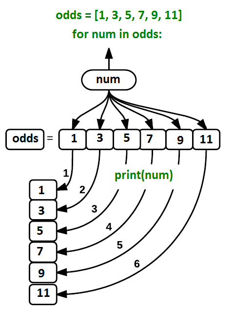
where each number (num) in the variable
odds is looped through and printed one number after
another. The other numbers in the diagram denote which loop cycle the
number was printed in (1 being the first loop cycle, and 6 being the
final loop cycle).
We can call the loop
variable anything we like, but there must be a colon at the end of
the line starting the loop, and we must indent anything we want to run
inside the loop. Unlike many other languages, there is no command to
signify the end of the loop body (e.g. end for); what is
indented after the for statement belongs to the loop.
What’s in a name?
In the example above, the loop variable was given the name
num as a mnemonic; it is short for ‘number’. We can choose
any name we want for variables. We might just as easily have chosen the
name banana for the loop variable, as long as we use the
same name when we invoke the variable inside the loop:
OUTPUT
1
3
5
7
9
11
It is a good idea to choose variable names that are meaningful, otherwise it would be more difficult to understand what the loop is doing.
Here’s another loop that repeatedly updates a variable:
PYTHON
length = 0
names = ['Curie', 'Darwin', 'Turing']
for value in names:
    length = length + 1
print('There are', length, 'names in the list.')
OUTPUT
There are 3 names in the list.It’s worth tracing the execution of this little program step by step.
Since there are three names in names, the statement on line
4 will be executed three times. The first time around,
length is zero (the value assigned to it on line 1) and
value is Curie. The statement adds 1 to the
old value of length, producing 1, and updates
length to refer to that new value. The next time around,
value is Darwin and length is 1,
so length is updated to be 2. After one more update,
length is 3; since there is nothing left in
names for Python to process, the loop finishes and the
print function on line 5 tells us our final answer.
Note that a loop variable is a variable that is being used to record progress in a loop. It still exists after the loop is over, and we can re-use variables previously defined as loop variables as well:
PYTHON
name = 'Rosalind'
for name in ['Curie', 'Darwin', 'Turing']:
    print(name)
print('after the loop, name is', name)
OUTPUT
Curie
Darwin
Turing
after the loop, name is Turing
Note also that finding the length of an object is such a common
operation that Python actually has a built-in function to do it called
len:
OUTPUT
4len is much faster than any function we could write
ourselves, and much easier to read than a two-line loop; it will also
give us the length of many other things that we haven’t met yet, so we
should always use it when we can.
From 1 to N
Python has a built-in function called range that
generates a sequence of numbers. range can accept 1, 2, or
3 parameters.
- If one parameter is given,
rangegenerates a sequence of that length, starting at zero and incrementing by 1. For example,range(3)produces the numbers0, 1, 2. - If two parameters are given,
rangestarts at the first and ends just before the second, incrementing by one. For example,range(2, 5)produces2, 3, 4. - If
rangeis given 3 parameters, it starts at the first one, ends just before the second one, and increments by the third one. For example,range(3, 10, 2)produces3, 5, 7, 9.
Using range, write a loop that uses range
to print the first 3 natural numbers:
OUTPUT
1
2
3The body of the loop is executed 6 times.
Summing a list
Write a loop that calculates the sum of elements in a list by adding
each element and printing the final value, so
[124, 402, 36] prints 562
Computing the Value of a Polynomial
The built-in function enumerate takes a sequence (e.g. a
list) and generates
a new sequence of the same length. Each element of the new sequence is a
pair composed of the index (0, 1, 2,…) and the value from the original
sequence:
The code above loops through a_list, assigning the index
to idx and the value to val.
Suppose you have encoded a polynomial as a list of coefficients in the following way: the first element is the constant term, the second element is the coefficient of the linear term, the third is the coefficient of the quadratic term, etc, where the polynomial is of the form
ax^0 + bx^1 + cx^2
(when writing polynomials mathematically, the x^0, is often omitted since this equals 1)
OUTPUT
97Write a loop using enumerate(coefs) which computes the
value y of any polynomial, given x and
coefs.
- “Use
for variable in sequenceto process the elements of a sequence one at a time.” - “The body of a
forloop must be indented.” - “Use
len(thing)to determine the length of something that contains other values.”
Content from Analyzing Data from Multiple Files
Last updated on 2026-01-13 | Edit this page
Overview
Questions
- “How can I do the same operations on many different files?”
Objectives
- “Use a library function to get a list of filenames that match a wildcard pattern.”
- “Write a
forloop to process multiple files.”
When working with real datasets, we may not always have everything in
a single file. We need a way to get a list of all the files in our
data directory whose names start with wave_
and end with .csv. The following library will help us to
achieve this:
The glob library contains a function, also called
glob, that finds files and directories whose names match a
pattern. We provide those patterns as strings: the character
* matches zero or more characters, while ?
matches any one character. We can use this to get the names of all the
CSV files in the current directory:
OUTPUT
['waves_10s.csv', 'waves_00s.csv', 'waves_80s.csv', 'waves_90s.csv']These files show waveheight data from some years in the decades
indicated in the filename. As this example shows,
glob.glob’s result is a list of files in arbitrary order.
This means we can loop over it to do something with each filename in
turn. In our case, the “something” we want to do is generate a set of
plots for each file in our waveheight dataset.
If we want to start by analyzing just the first three files in
alphabetical order, we can use the sorted built-in function
to generate a new sorted list from the glob.glob
output:
PYTHON
import glob
import numpy
import matplotlib.pyplot as plt

filenames = sorted(glob.glob('waves_*.csv'))
filenames = filenames[0:3]

for filename in filenames:
    print(filename)

    data = numpy.loadtxt(fname=filename, delimiter=',')
    number_of_rows = data.shape[0]
    number_of_years = number_of_rows//12

    # need to reshape the data for plotting
    data = numpy.reshape(data[:,2], [number_of_years,12])

    fig = plt.figure(figsize=(10.0, 3.0))

    axes1 = fig.add_subplot(1, 3, 1)
    axes2 = fig.add_subplot(1, 3, 2)
    axes3 = fig.add_subplot(1, 3, 3)

    axes1.set_ylabel('average')
    axes1.plot(numpy.mean(data, axis=0))

    axes2.set_ylabel('max')
    axes2.plot(numpy.max(data, axis=0))

    axes3.set_ylabel('min')
    axes3.plot(numpy.min(data, axis=0))

    fig.tight_layout()
    plt.show()
OUTPUT
waves_00.csv
OUTPUT
waves_10s.csv
OUTPUT
waves_80s.csv
Looking at these three decades, we can see similarities - with the average value representing a smooth climate with clear annual cycle. There are differences year on year, and the minimum and maximum data tend to be more variable than the mean.
Different types of division
You might have noticed that we calculated the number of years when reshaping the data, rather than using 10 years for each decade. This was useful here because the file containing data from the 2010s only has data from 6 years, but each one of these years did contain data for every month. If any year had missing data from any month, we would have needed to have done some additional preprocessing.
When we divided by 12 to get the number of years, we used
// - you might have expected us just to use /.
Python creates a float as a result from a division operation using
/, even if both inputs are integers:
OUTPUT
floatHowever, if you use a float value as an array index, you get an error
(even if it refers to a whole number). // is Python’s
integer division operator - meaning that the result will always be an
integer:
OUTPUT
intIf the result would normally result in a floating-point number, the actual result will instead be an integer rounded towards minus infinity:
OUTPUT
4.75
4
Sometimes, plots can help us spot patterns in data, or problems with data.
Let’s load waves_90s.csv and reshape it so that the 3rd
column (the average signifncant wave height for each month) is converted
into 12 columns for each year.
PYTHON
data = numpy.loadtxt(fname = "waves_90s.csv", delimiter=',')
reshaped_data = numpy.reshape(data[:,2], [10,12])
print(data.shape)
print(reshaped_data.shape)
OUTPUT
(120, 3)
(10, 12)
If we try and take the mean for the entire year, we’ll see that there must be NaNs:
OUTPUT
np.float64(nan)If we plot the reshaped data, we would see white squares where there are NaNs in the data. Let’s do the shaping operation again but this time in a more generic way where we don’t need to know how many years are represented in the dataset.
PYTHON
number_of_rows = data.shape[0]
# assume that every 12 rows represents one year of data and there's no missing data
number_of_years = number_of_rows//12
data = numpy.reshape(data[:,2], [number_of_years,12])
plt.imshow(data)
plt.show()
We can clearly see that there must have been some problem with the collection of data in the first 6 months of 1994. Apart from that, the rest of the data looks relatively sensible, with low wave heights in the summer months of the decade, and higher wave heights in the winter months of the decade. This means that we have no reason not to trust the rest of the dataset.
There are other ways that we could have determined where the missing
data is. The Numpy function isnan will tell us whether any
given value is NaN; if we give it an ndarray, it will
return an ndarray of the same shape with boolean values
(True or False) showing if the value at that
index was a NaN. argwhere will return the indices for an
ndarray of booleans where the value is
True.
OUTPUT
array([[4, 0],
       [4, 1],
       [4, 2],
       [4, 3],
       [4, 4],
       [4, 5]])
There are almost always multiple ways to achieve the same result in programming, and often the choice as to which method to use comes down to personal preference. Some people might prefer to look at patterns in plots, while others may be happy to look at summary statistics and aggregate values from tabular data to come to the same conclusion.
Plotting Differences
Plot the difference between the average monthly waveheights in the 1980s and 1990s. Can you do this using glob, without specifying the filenames explicitly in the code?
PYTHON
import glob
import numpy
import matplotlib.pyplot as plt

filenames = sorted(glob.glob('waves_*.csv'))

data0 = numpy.loadtxt(fname=filenames[2], delimiter=',')
data1 = numpy.loadtxt(fname=filenames[3], delimiter=',')

number_of_rows0 = data0.shape[0]
number_of_years0 = number_of_rows0//12
data0 = numpy.reshape(data0[:,2], [number_of_years0,12])

number_of_rows1 = data1.shape[0]
number_of_years1 = number_of_rows1//12
data1 = numpy.reshape(data1[:,2], [number_of_years1,12])

fig = plt.figure(figsize=(10.0, 3.0))

plt.ylabel('Difference in average')
plt.plot(numpy.mean(data0, axis=0) - numpy.mean(data1, axis=0))

fig.tight_layout()
plt.show()
Congratulations! We’ve investigated the wave data and spotted some trends, and identified bad / missing data. Now that we understand what is in the model data set, and trust that it is realistic, we can use it to make practical decisions about things like boat operations
- “Use
glob.glob(pattern)to create a list of files whose names match a pattern.” - “Use
*in a pattern to match zero or more characters, and?to match any single character.”
Content from Making Choices
Last updated on 2026-01-13 | Edit this page
Overview
Questions
- “How can my programs do different things based on data values?”
Objectives
- “Write conditional statements including
if,elif, andelsebranches.” - “Correctly evaluate expressions containing
andandor.”
In our previous lessons, we examined the seasonal behaviour of sea waves. How can we use this data to make practical decisions?
How can we use Python to identify thresholds, and take a different action for each? In this lesson, we’ll learn how to write code that runs only when certain conditions are true.
Conditionals
We can ask Python to take different actions, depending on a
condition, with an if statement:
OUTPUT
not greater
done
The second line of this code uses the keyword if to tell
Python that we want to make a choice. If the test that follows the
if statement is true, the body of the if
(i.e., the set of lines indented underneath it) is executed, and
“greater” is printed. If the test is false, the body of the
else is executed instead, and “not greater” is printed.
Only one or the other is ever executed before continuing on with program
execution to print “done”:

Conditional statements don’t have to include an else. If
there isn’t one, Python simply does nothing if the test is false:
PYTHON
num = 53
print('before conditional...')
if num > 100:
    print(num, "is greater than 100")
print('...after conditional')
OUTPUT
before conditional...
...after conditional
We can also chain several tests together using elif,
which is short for “else if”. The following Python code uses
elif to print the sign of a number.
PYTHON
num = -3

if num > 0:
    print(num, "is positive")
elif num == 0:
    print(num, "is zero")
else:
    print(num, "is negative")
OUTPUT
-3 is negativeNote that to test for equality we use a double equals sign
== rather than a single equals sign = which is
used to assign values.
Comparing in Python
Along with the > and == operators we
have already used for comparing values in our conditionals, there are a
few more options to know about:
-
>: greater than -
<: less than -
==: equal to -
!=: does not equal -
>=: greater than or equal to -
<=: less than or equal to
We can also combine tests using and and or.
and is only true if both parts are true:
PYTHON
if (1 > 0) and (-1 >= 0):
    print("both parts are true")
else:
    print("at least one part is false")
OUTPUT
at least one part is falsewhile or is true if at least one part is true:
OUTPUT
at least one test is true
True and False
True and False are special words in Python
called booleans, which represent truth values. A statement
such as 1 < 0 returns the value False,
while -1 < 0 returns the value True.
Checking our Data
Now that we’ve seen how conditionals work, we can use them to look
for thresholds in our wave data. We are about to use functions provided
by the numpy module again. Therefore, if you’re working in
a new Python session, make sure to load the module again:
If you are operating a boat, for carrying passengers of working offshore, you need to know that it will be save to go to sea. Ideally you wouldn’t want to have passengers transported if the wave height is above 3 metres
Let’s look at our wave data, and find which months we can operate the boats, based on the monthly mean wave-height.
We could look at each month individually:
PYTHON
data = numpy.loadtxt(fname='data/wavesmonthly.csv', delimiter=',', skiprows=1)
reshaped_data = numpy.reshape(data[:,2], [37,12])

month0 = numpy.mean(reshaped_data, axis=0)[0]

if month0 < 3:
    print("Can take passengers this month")
Survey vehicles can operate in stormier waters, with wave heights up to 4m
And if neither of these conditions are true, then it’s too stormy, and nothing can go out.
Let’s test that out for February:
PYTHON
month1 = numpy.mean(reshaped_data, axis=0)[1]
if month1 < 3:
print("Can take passengers this month")
elif month1 < 4:
print("Can take survey vehicles (but not passengers)")
else:
print("Can't take any boats out to sea")OUTPUT
Can't take any boats out to seaNow let’s try for June
PYTHON
month5 = numpy.mean(reshaped_data, axis=0)[5]

if month5 < 3:
    print("Can take passengers this month")
elif month5 < 4:
    print("Can take survey vehicles (but not passengers)")
else:
    print("Can't take any boats out to sea")
OUTPUT
Can take passengers this monthNotice how the statement stops as soon as it reaches a condition
which is True.
We could test for all months less manually, using a
for loop:
PYTHON
for month_index, monthly_waveheight in enumerate(numpy.mean(reshaped_data, axis=0)):
    if monthly_waveheight < 3:
        print(f"Month {month_index}: we can take passengers this month")
    elif monthly_waveheight < 4:
        print(f"Month {month_index}: we can take survey vehicles (but not passengers) this month")
    else:
        print(f"Month {month_index}: we can't take any boats out to sea this month")
OUTPUT
Month 0: can't take any boats out to sea this month
Month 1: can't take any boats out to sea this month
Month 2: can't take any boats out to sea this month
Month 3: can take survey vehicles (but not passengers) this month
Month 4: can take passengers this month
Month 5: can take passengers this month
Month 6: can take passengers this month
Month 7: can take passengers this month
Month 8: can take passengers this month
Month 9: can take survey vehicles (but not passengers) this month
Month 10: can take survey vehicles (but not passengers) this month
Month 11: can't take any boats out to sea this month
The enumerate function is the Pythonic way of
getting the index of values in a loop - in this case it allows us to
list the month number in the output. We need a variable to store this
value in, which we’re calling month_index. Because the loop
returns two variables form each iteration (month index and monthly
waveheight), we need two variables.
We can see that we could suggest a timetable for passenger ferries in May - September (inclusive), we could plan to take survey boats out in April, October, and November; and we should not plan any sea-going activities in January, February, March, or December.
This is a relatively crude example, but shows how we can use these programming constructs to help make some decisions using the data.
In this way, we have asked Python to do something different depending
on the condition of our data. Here we printed messages in all cases, but
we could also imagine not using the else catch-all so that
messages are only printed when something is wrong, freeing us from
having to manually examine every plot for features we’ve seen
before.
C gets printed because the first two conditions,
4 > 5 and 4 == 5, are not true, but
4 < 5 is true.
What Is Truth?
True and False booleans are not the only
values in Python that are true and false. In fact, any value
can be used in an if or elif. After reading
and running the code below, explain what the rule is for which values
are considered true and which are considered false.
OUTPUT
word is true
non-empty list is true
one is true
A non-empty string, non-empty list and non-zero variable all evaluate to True. An empty string, empty list and zero all evaluate to False.
That’s Not Not What I Meant
Sometimes it is useful to check whether some condition is not true.
The Boolean operator not can do this explicitly. After
reading and running the code below, write some if
statements that use not to test the rule that you
formulated in the previous challenge.
OUTPUT
empty string is not true
not not True is true
The not of an empty string evaluates to True. Evaluating not twice converts back to original value, so doing not twice on True is True.
Close Enough
Write some conditions that print True if the variable
a is within 10% of the variable b and
False otherwise. Compare your implementation with your
partner’s: do you get the same answer for all possible pairs of
numbers?
There is a built-in
function abs that returns the absolute value of a
number:
OUTPUT
12In-Place Operators
Python (and most other languages in the C family) provides in-place operators that work like this:
PYTHON
x = 1  # original value
x += 1 # add one to x, assigning result back to x
x *= 3 # multiply x by 3
print(x)
OUTPUT
6Write some code that sums the positive and negative numbers in a list separately, using in-place operators. Do you think the result is more or less readable than writing the same without in-place operators?
PYTHON
positive_sum = 0
negative_sum = 0
test_list = [3, 4, 6, 1, -1, -5, 0, 7, -8]
for num in test_list:
    if num 0:
        positive_sum += num
    elif num == 0:
        pass
    else:
        negative_sum += num
print(positive_sum, negative_sum)
Here pass means “don’t do anything”. In this particular
case, it’s not actually needed, since if num == 0 neither
sum needs to change, but it illustrates the use of elif and
pass.
Sorting a List Into Buckets
In our data folder, we have some CSV files (those with
.csv file extensions), and one NetCDF file (with a .nc file extension).
We’d like to break these files into two lists called
csv_files and nc_files, respectively.
Add code to the template below to do this. Note that the string
method startswith
returns True if and only if the string it is called on ends
with the string passed as an argument, that is:
OUTPUT
TrueBut
OUTPUT
FalseUse the following Python code as your starting point:
PYTHON
filenames = ['wavesmonthly.csv',
         'waves_00s.csv',
         'waves_10s.csv',
         'waves_80s.csv',
         'waves_90s.csv',
         'multyear_hs_avg.nc']
csv_files = []
nc_files = []
other_files = []
Your solution should:
- loop over the names of the files
- figure out which group each filename belongs in
- append the filename to that list
In the end the two lists should be:
PYTHON
filenames = ['wavesmonthly.csv',
        'waves_00s.csv',
        'waves_10s.csv',
        'waves_80s.csv',
        'waves_90s.csv',
        'multyear_hs_avg.nc']
csv_files = []
nc_files = []
other_files = []

for filename in filenames:
    if filename.endswith('csv'):
        csv_files.append(filename)
    elif filename.endswith('nc'):
        nc_files.append(filename)
    else:
        other_files.append(filename)

print("csv_files:", csv_files)
print("nc_files:", nc_files)
print("other_files:", other_files)
OUTPUT
csv_files: ['wavesmonthly.csv', 'waves_00s.csv', 'waves_10s.csv', 'waves_80s.csv', 'waves_90s.csv']
nc_files: ['multyear_hs_avg.nc']
other_files: []Counting Vowels
- Write a loop that counts the number of vowels in a character string.
- Test it on a few individual words and full sentences.
- Once you are done, compare your solution to your neighbor’s. Did you make the same decisions about how to handle the letter ‘y’ (which some people think is a vowel, and some do not)?
- “Use
if conditionto start a conditional statement,elif conditionto provide additional tests, andelseto provide a default.” - “The bodies of the branches of conditional statements must be indented.”
- “Use
==to test for equality.” - “
X and Yis only true if bothXandYare true.” - “
X or Yis true if eitherXorY, or both, are true.” - “Zero, the empty string, and the empty list are considered false; all other numbers, strings, and lists are considered true.”
- “
TrueandFalserepresent truth values.”
Content from Creating Functions
Last updated on 2026-01-13 | Edit this page
Overview
Questions
- “How can I define new functions?”
- “What’s the difference between defining and calling a function?”
- “What happens when I call a function?”
Objectives
- “Define a function that takes parameters.”
- “Return a value from a function.”- “Test and debug a function.”
- “Set default values for function parameters.”
- “Explain why we should divide programs into small, single-purpose functions.”
At this point, we’ve written code to draw some interesting features
in our wave data, loop over all our data files to quickly draw these
plots for each of them, and have Python make decisions based on what it
sees in our data. But, our code is getting pretty long and complicated;
what if we had thousands of datasets, and didn’t want to generate a
figure for every single one? Commenting out the figure-drawing code is a
nuisance. Also, what if we want to use that code again, on a different
dataset or at a different point in our program? Cutting and pasting it
is going to make our code get very long and very repetitive, very
quickly. We’d like a way to package our code so that it is easier to
reuse, and Python provides for this by letting us define things called
‘functions’ — a shorthand way of re-executing longer pieces of code.
Let’s start by defining a function fahr_to_celsius that
converts temperatures from Fahrenheit to Celsius:

The function definition opens with the keyword def
followed by the name of the function (fahr_to_celsius) and
a parenthesized list of parameter names (temp). The body of the function — the statements
that are executed when it runs — is indented below the definition line.
The body concludes with a return keyword followed by the
return value.
When we call the function, the values we pass to it are assigned to those variables so that we can use them inside the function. Inside the function, we use a return statement to send a result back to whoever asked for it.
Let’s try running our function.
This command should call our function, using “32” as the input and return the function value.
In fact, calling our own function is no different from calling any other function:
PYTHON
print('freezing point of water:', fahr_to_celsius(32), 'C')
print('boiling point of water:', fahr_to_celsius(212), 'C')
OUTPUT
freezing point of water: 0.0 C
boiling point of water: 100.0 C
We’ve successfully called the function that we defined, and we have access to the value that we returned.
Composing Functions
Now that we’ve seen how to turn Fahrenheit into Celsius, we can also write the function to turn Celsius into Kelvin:
PYTHON
def celsius_to_kelvin(temp_c):
    return temp_c + 273.15

print('freezing point of water in Kelvin:', celsius_to_kelvin(0.))
OUTPUT
freezing point of water in Kelvin: 273.15What about converting Fahrenheit to Kelvin? We could write out the formula, but we don’t need to. Instead, we can compose the two functions we have already created:
PYTHON
def fahr_to_kelvin(temp_f):
    temp_c = fahr_to_celsius(temp_f)
    temp_k = celsius_to_kelvin(temp_c)
    return temp_k

print('boiling point of water in Kelvin:', fahr_to_kelvin(212.0))
OUTPUT
boiling point of water in Kelvin: 373.15This is our first taste of how larger programs are built: we define basic operations, then combine them in ever-larger chunks to get the effect we want. Real-life functions will usually be larger than the ones shown here — typically half a dozen to a few dozen lines — but they shouldn’t ever be much longer than that, or the next person who reads it won’t be able to understand what’s going on.
Variable Scope
In composing our temperature conversion functions, we created
variables inside of those functions, temp,
temp_c, temp_f, and temp_k. We
refer to these variables as local variables because they no
longer exist once the function is done executing. If we try to access
their values outside of the function, we will encounter an error:
ERROR
---------------------------------------------------------------------------
NameError                                 Traceback (most recent call last)
<ipython-input-1-eed2471d229bin <module>
----1 print('Again, temperature in Kelvin was:', temp_k)

NameError: name 'temp_k' is not defined
If you want to reuse the temperature in Kelvin after you have
calculated it with fahr_to_kelvin, you can store the result
of the function call in a variable:
OUTPUT
temperature in Kelvin was: 373.15The variable temp_kelvin, being defined outside any
function, is said to be global.
Inside a function, one can read the value of such global variables:
PYTHON
def print_temperatures():
  print('temperature in Fahrenheit was:', temp_fahr)
  print('temperature in Kelvin was:', temp_kelvin)

temp_fahr = 212.0
temp_kelvin = fahr_to_kelvin(temp_fahr)

print_temperatures()
OUTPUT
temperature in Fahrenheit was: 212.0
temperature in Kelvin was: 373.15
Tidying up
Now that we know how to wrap bits of code up in functions, we can
make our wave data easier to read and easier to reuse. First, let’s make
a visualize function that generates our plots:
PYTHON
import numpy as np
def visualize(filename):
    data = np.loadtxt(fname=filename, delimiter=',')
    number_of_rows = data.shape[0] # total number of months
    number_of_years = number_of_rows // 12 # total number of years = number of months / number of months per year

    # need to reshape the data for plotting
    reshaped_data = np.reshape(data[:,2], [number_of_years,12])

    fig = matplotlib.pyplot.figure(figsize=(10.0, 3.0))

    axes1 = fig.add_subplot(1, 3, 1)
    axes2 = fig.add_subplot(1, 3, 2)
    axes3 = fig.add_subplot(1, 3, 3)

    axes1.set_ylabel('average')
    axes1.plot(np.mean(reshaped_data, axis=0))

    axes2.set_ylabel('max')
    axes2.plot(np.max(reshaped_data, axis=0))

    axes3.set_ylabel('min')
    axes3.plot(np.min(reshaped_data, axis=0))

    fig.tight_layout()
    matplotlib.pyplot.show()
Wait! Didn’t we forget to specify what this function should return?
Well, we didn’t. In Python, functions are not required to include a
return statement and can be used for the sole purpose of
grouping together pieces of code that conceptually do one thing. In such
cases, function names usually describe what they do, e.g.
visualize.
Notice that rather than jumbling this code together in one giant
for loop, we can now read and reuse the code. We can
reproduce the previous analysis with a much simpler for
loop:
PYTHON
import glob
filenames = sorted(glob.glob('waves_*.csv'))

for filename in filenames[1:3]:
    print(filename)
    visualize(filename)
By giving our functions human-readable names, we can more easily read
and understand what is happening in the for loop. Even
better, if at some later date we want to use either of those pieces of
code again, we can do so in a single line.
Testing and Documenting
Once we start putting things in functions so that we can re-use them, we need to start testing that those functions are working correctly. To see how to do this, let’s write a function to offset a dataset so that it’s mean value shifts to a user-defined value:
We could test this on our actual data, but since we don’t know what the values ought to be, it will be hard to tell if the result was correct. Instead, let’s use NumPy to create a matrix of 0’s and then offset its values to have a mean value of 3:
OUTPUT
[[ 3. 3.]
[ 3. 3.]]That looks right, so let’s try offset_mean on our real
data:
PYTHON
reshaped_data = np.loadtxt(fname='reshaped_data.csv', delimiter=',')
print(offset_mean(reshaped_data, 0))OUTPUT
[[ 4.04436937e-01 3.84436937e-01 1.39043694e+00 -5.65563063e-01
-6.49563063e-01 -1.29756306e+00 -1.31756306e+00 -1.14756306e+00
-6.15630631e-02 1.28436937e-01 9.64436937e-01 1.24443694e+00]
...
[ 3.10443694e+00 2.57043694e+00 8.76436937e-01 2.45443694e+00
1.49843694e+00 2.94436937e-01 -7.55630631e-02 -5.97563063e-01
-6.73563063e-01 -3.37563063e-01 1.23843694e+00 1.66443694e+00]]It’s hard to tell from the default output whether the result is correct, but there are a few tests that we can run to reassure us:
PYTHON
print('original min, mean, and max are:', np.min(reshaped_data), np.mean(reshaped_data), np.max(reshaped_data))
offset_data = offset_mean(reshaped_data, 0)
print('min, mean, and max of offset data are:',
np.min(offset_data),
np.mean(offset_data),
np.max(offset_data))OUTPUT
original min, mean, and max are: 1.496 3.383563063063063 6.956
min, mean, and max of offset data are: -1.8875630630630629 1.960393809248024e-16 3.5724369369369375That seems almost right: the original mean was about 1.5, so the lower bound from zero is now about -1.9. The mean of the offset data isn’t quite zero — we’ll explore why not in the challenges — but it’s pretty close. We can even go further and check that the standard deviation hasn’t changed:
OUTPUT
std dev before and after: 1.1440155050316319 1.144015505031632Those values look the same, but we probably wouldn’t notice if they were different in the sixth decimal place. Let’s do this instead:
PYTHON
print('difference in standard deviations before and after:',
np.std(data) - np.std(offset_data))OUTPUT
difference in standard deviations before and after: -2.220446049250313e-16Again, the difference is very small. It’s still possible that our function is wrong, but it seems unlikely enough that we should probably get back to doing our analysis. We have one more task first, though: we should write some documentation for our function to remind ourselves later what it’s for and how to use it.
The usual way to put documentation in software is to add comments like this:
PYTHON
# offset_mean(data, target_mean_value):
# return a new array containing the original data with its mean offset to match the desired value.
def offset_mean(data, target_mean_value):
return (data - np.mean(data)) + target_mean_valueThere’s a better way, though. If the first thing in a function is a string that isn’t assigned to a variable, that string is attached to the function as its documentation:
PYTHON
def offset_mean(data, target_mean_value):
"""Return a new array containing the original data
with its mean offset to match the desired value."""
return (data - np.mean(data)) + target_mean_valueThis is better because we can now ask Python’s built-in help system to show us the documentation for the function:
OUTPUT
Help on function offset_mean in module __main__:
offset_mean(data, target_mean_value)
Return a new array containing the original data with its mean offset to match the desired value.A string like this is called a docstring. We don’t need to use triple quotes when we write one, but if we do, we can break the string across multiple lines:
PYTHON
def offset_mean(data, target_mean_value):
"""Return a new array containing the original data
with its mean offset to match the desired value.
Examples
--------
>>offset_mean([1, 2, 3], 0)
array([-1., 0., 1.])
"""
return (data - np.mean(data)) + target_mean_value
help(offset_mean)OUTPUT
Help on function offset_mean in module __main__:
offset_mean(data, target_mean_value)
Return a new array containing the original data
with its mean offset to match the desired value.
Examples
--------
>>offset_mean([1, 2, 3], 0)
array([-1., 0., 1.])Defining Defaults
We have passed parameters to functions in two ways: directly, as in
type(data), and by name, as in
np.loadtxt(fname='something.csv', delimiter=','). In fact,
we can pass the filename to loadtxt without the
fname=:
OUTPUT
array([[3.788, 3.768, 4.774, 2.818, 2.734, 2.086, 2.066, 2.236, 3.322,
3.512, 4.348, 4.628],
[3.666, 4.326, 3.522, 3.18 , 1.954, 1.72 , 1.86 , 1.95 , 3.11 ,
3.78 , 3.474, 5.28 ],
[5.068, 4.954, 3.77 , 2.402, 2.166, 2.084, 2.246, 2.228, 2.634,
4.41 , 4.342, 3.28 ],
...,
[4.27 , 4.09 , 3.696, 3.302, 2.502, 1.772, 2.016, 2.172, 3.034,
3.462, 3.856, 5.76 ],
[4.294, 3.794, 4.646, 3.212, 2.226, 1.558, 1.894, 2.092, 2.58 ,
3.87 , 3.108, 6.044],
[6.488, 5.954, 4.26 , 5.838, 4.882, 3.678, 3.308, 2.786, 2.71 ,
3.046, 4.622, 5.048]])but we still need to say delimiter=',':
ERROR
Traceback (most recent call last):
File ~/mambaforge/envs/python-workshop/lib/python3.11/site-packages/IPython/core/interactiveshell.py:3579 in run_code
exec(code_obj, self.user_global_ns, self.user_ns)
Cell In[26], line 1
np.loadtxt('reshaped_data.csv', ',')
File /Users/username/anaconda3/lib/python3.6/site-packages/numpy/lib/_npyio_impl.py:1395 in loadtxt
arr = _read(fname, dtype=dtype, comment=comment, delimiter=delimiter,
File /Users/username/anaconda3/lib/python3.6/site-packages/numpy/lib/_npyio_impl.py:947 in _read
dtype = np.dtype(dtype)
File /Users/username/anaconda3/lib/python3.6/site-packages/numpy/_core/_internal.py:204 in _commastring
newitem = (dtype, ast.literal_eval(repeats))
File /Users/username/anaconda3/lib/python3.6/ast.py:64 in literal_eval
node_or_string = parse(node_or_string.lstrip(" \t"), mode='eval')
File /Users/username/anaconda3/lib/python3.6/ast.py:50 in parse
return compile(source, filename, mode, flags,
File <unknown>:1
,
^
SyntaxError: invalid syntaxTo understand what’s going on, and make our own functions easier to
use, let’s re-define our offset_mean function like
this:
PYTHON
def offset_mean(data, target_mean_value=0.0):
"""Return a new array containing the original data
with its mean offset to match the desired value, (0 by default).
Examples
--------
>>offset_mean([1, 2, 3])
array([-1., 0., 1.])
"""
return (data - np.mean(data)) + target_mean_valueThe key change is that the second parameter is now written
target_mean_value=0.0 instead of just
target_mean_value. If we call the function with two
arguments, it works as it did before:
[[ 3.  3.]
[ 3. 3.]]But we can also now call it with just one parameter, in which case
target_mean_value is automatically assigned the default value of 0.0:
PYTHON
more_data = 5 + np.zeros((2, 2))
print('data before mean offset:')
print(more_data)
print('offset data:')
print(offset_mean(more_data))
OUTPUT
data before mean offset:
[[ 5.  5.]
 [ 5.  5.]]
offset data:
[[ 0.  0.]
 [ 0.  0.]]
This is handy: if we usually want a function to work one way, but occasionally need it to do something else, we can allow people to pass a parameter when they need to but provide a default to make the normal case easier. The example below shows how Python matches values to parameters:
PYTHON
def display(a=1, b=2, c=3):
    print('a:', a, 'b:', b, 'c:', c)

print('no parameters:')
display()
print('one parameter:')
display(55)
print('two parameters:')
display(55, 66)
OUTPUT
no parameters:
a: 1 b: 2 c: 3
one parameter:
a: 55 b: 2 c: 3
two parameters:
a: 55 b: 66 c: 3
As this example shows, parameters are matched up from left to right, and any that haven’t been given a value explicitly get their default value. We can override this behavior by naming the value as we pass it in:
OUTPUT
only setting the value of c
a: 1 b: 2 c: 77
With that in hand, let’s look at the help for
np.loadtxt:
OUTPUT
Help on function loadtxt in module numpy.lib.npyio:

loadtxt(fname, dtype=<class 'float'>, comments='#', delimiter=None, converters=None, skiprows=0, use
cols=None, unpack=False, ndmin=0, encoding='bytes')
    Load data from a text file.

    Each row in the text file must have the same number of values.

    Parameters
    ----------
...
There’s a lot of information here, but the most important part is the first couple of lines:
PYTHON
loadtxt(fname, dtype=<class 'float'>, comments='#', delimiter=None, converters=None, skiprows=0, use
cols=None, unpack=False, ndmin=0, encoding='bytes')
This tells us that loadtxt has one parameter called
fname that doesn’t have a default value, and eight others
that do. If we call the function like this:
then the filename is assigned to fname (which is what we
want), but the delimiter string ',' is assigned to
dtype rather than delimiter, because
dtype is the second parameter in the list. However
',' isn’t a known dtype so our code produced
an error message when we tried to run it. When we call
loadtxt we don’t have to provide fname= for
the filename because it’s the first item in the list, but if we want the
',' to be assigned to the variable delimiter,
we do have to provide delimiter= for the second
parameter since delimiter is not the second parameter in
the list.
Readable functions
Consider these two functions:
PYTHON
def s(p):
    a = 0
    for v in p:
        a += v
    m = a / len(p)
    d = 0
    for v in p:
        d += (v - m) * (v - m)
    return np.sqrt(d / (len(p) - 1))

def std_dev(sample):
    sample_sum = 0
    for value in sample:
        sample_sum += value

    sample_mean = sample_sum / len(sample)

    sum_squared_devs = 0
    for value in sample:
        sum_squared_devs += (value - sample_mean) * (value - sample_mean)

    return np.sqrt(sum_squared_devs / (len(sample) - 1))
The functions s and std_dev are
computationally equivalent (they both calculate the sample standard
deviation), but to a human reader, they look very different. You
probably found std_dev much easier to read and understand
than s.
As this example illustrates, both documentation and a programmer’s coding style combine to determine how easy it is for others to read and understand the programmer’s code. Choosing meaningful variable names and using blank spaces to break the code into logical “chunks” are helpful techniques for producing readable code. This is useful not only for sharing code with others, but also for the original programmer. If you need to revisit code that you wrote months ago and haven’t thought about since then, you will appreciate the value of readable code!
Combining Strings
“Adding” two strings produces their concatenation:
'a' + 'b' is 'ab'. Write a function called
fence that takes two parameters called
original and wrapper and returns a new string
that has the wrapper character at the beginning and end of the original.
A call to your function should look like this:
OUTPUT
*name*Return versus print
Note that return and print are not
interchangeable. print is a Python function that
prints data to the screen. It enables us, users, see
the data. return statement, on the other hand, makes data
visible to the program. Let’s have a look at the following function:
Question: What will we see if we execute the following commands?
Python will first execute the function add with
a = 7 and b = 3, and, therefore, print
10. However, because function add does not
have a line that starts with return (no return
“statement”), it will, by default, return nothing which, in Python
world, is called None. Therefore, A will be
assigned to None and the last line (print(A))
will print None. As a result, we will see:
OUTPUT
10
NoneSelecting Characters From Strings
If the variable s refers to a string, then
s[0] is the string’s first character and s[-1]
is its last. Write a function called outer that returns a
string made up of just the first and last characters of its input. A
call to your function should look like this:
OUTPUT
hmRescaling an Array
Write a function rescale that takes an array as input
and returns a corresponding array of values scaled to lie in the range
0.0 to 1.0. (Hint: If L and H are the lowest
and highest values in the original array, then the replacement for a
value v should be (v-L) / (H-L).)
Testing and Documenting Your Function
Run the commands help(np.arange) and
help(np.linspace) to see how to use these functions to
generate regularly-spaced values, then use those values to test your
rescale function. Once you’ve successfully tested your
function, add a docstring that explains what it does.
PYTHON
"""Takes an array as input, and returns a corresponding array scaled so
that 0 corresponds to the minimum and 1 to the maximum value of the input array.

Examples:
>>rescale(np.arange(10.0))
array([ 0.        ,  0.11111111,  0.22222222,  0.33333333,  0.44444444,
       0.55555556,  0.66666667,  0.77777778,  0.88888889,  1.        ])
>>rescale(np.linspace(0, 100, 5))
array([ 0.  ,  0.25,  0.5 ,  0.75,  1.  ])
"""Defining Defaults
Rewrite the rescale function so that it scales data to
lie between 0.0 and 1.0 by default, but will
allow the caller to specify lower and upper bounds if they want. Compare
your implementation to your neighbor’s: do the two functions always
behave the same way?
PYTHON
def rescale(input_array, low_val=0.0, high_val=1.0):
    """rescales input array values to lie between low_val and high_val"""
    L = np.min(input_array)
    H = np.max(input_array)
    intermed_array = (input_array - L) / (H - L)
    output_array = intermed_array * (high_val - low_val) + low_val
return output_arrayOUTPUT
259.81666666666666
278.15
273.15
0
k is 0 because the k inside the function
f2k doesn’t know about the k defined outside
the function. When the f2k function is called, it creates a
local variable
k. The function does not return any values and does not
alter k outside of its local copy. Therefore the original
value of k remains unchanged. Beware that a local
k is created because f2k internal statements
affect a new value to it. If k was only
read, it would simply retrieve the global k
value.
Mixing Default and Non-Default Parameters
Given the following code:
PYTHON
def numbers(one, two=2, three, four=4):
n = str(one) + str(two) + str(three) + str(four)
return n
print(numbers(1, three=3))what do you expect will be printed? What is actually printed? What rule do you think Python is following?
1234one2three41239SyntaxError
Given that, what does the following piece of code display when run?
a: b: 3 c: 6a: -1 b: 3 c: 6a: -1 b: 2 c: 6a: b: -1 c: 2
Attempting to define the numbers function results in
4. SyntaxError. The defined parameters two and
four are given default values. Because one and
three are not given default values, they are required to be
included as arguments when the function is called and must be placed
before any parameters that have default values in the function
definition.
The given call to func displays
a: -1 b: 2 c: 6. -1 is assigned to the first parameter
a, 2 is assigned to the next parameter b, and
c is not passed a value, so it uses its default value
6.
Readable Code
Revise a function you wrote for one of the previous exercises to try to make the code more readable. Then, collaborate with one of your neighbors to critique each other’s functions and discuss how your function implementations could be further improved to make them more readable.
- “Define a function using
def function_name(parameter).” - “The body of a function must be indented.”
- “Call a function using
function_name(value).” - “Numbers are stored as integers or floating-point numbers.”
- “Variables defined within a function can only be seen and used within the body of the function.”
- “Variables created outside of any function are called global variables.”
- “Within a function, we can access global variables.”
- “Variables created within a function override global variables if their names match.”
- “Use
help(thing)to view help for something.” - “Put docstrings in functions to provide help for that function.”
- “Specify default values for parameters when defining a function
using
name=valuein the parameter list.” - “Parameters can be passed by matching based on name, by position, or by omitting them (in which case the default value is used).”
- “Put code whose parameters change frequently in a function, then call it with different parameter values to customize its behavior.”