Analyzing some wave-height data

Overview

Questions

• “How can I process tabular data files in Python?”

Objectives

• “Explain what a library is and what libraries are used for.”
• “Import a Python library and use the functions it contains.”
• “Read tabular data from a file into a program.”
• “Select individual values and subsections from data.”
• “Perform operations on arrays of data.”

Words are useful, but what’s more useful are the sentences and stories we build with them. Similarly, while a lot of powerful, general tools are built into Python, specialized tools built up from these basic units live in libraries that can be called upon when needed.

Loading data into Python

---

To begin processing the wavedata, we need to load it into Python. We can do that using a library called NumPy, which stands for Numerical Python. In general, you should use this library when you want to do fancy things with lots of numbers, especially if you have matrices or arrays. To tell Python that we’d like to start using NumPy, we need to import it:

PYTHON

import numpy

Importing a library is like getting a piece of lab equipment out of a storage locker and setting it up on the bench. Libraries provide additional functionality to the basic Python package, much like a new piece of equipment adds functionality to a lab space. Just like in the lab, importing too many libraries can sometimes complicate and slow down your programs - so we only import what we need for each program.

Once we’ve imported the library, we can ask the library to read our data file for us:

PYTHON

numpy.loadtxt(fname='wavesmonthly.csv', delimiter=',', skiprows=1)

OUTPUT

array([[1.979e+03, 1.000e+00, 3.788e+00],
       [1.979e+03, 2.000e+00, 3.768e+00],
       [1.979e+03, 3.000e+00, 4.774e+00],
       ...,
       [2.015e+03, 1.000e+01, 3.046e+00],
       [2.015e+03, 1.100e+01, 4.622e+00],
       [2.015e+03, 1.200e+01, 5.048e+00]], shape=(444, 3))

The expression numpy.loadtxt(...) is a function call that asks Python to run the function loadtxt which belongs to the numpy library. The dot notation in Python is used most of all as an object attribute/property specifier or for invoking its method. object.property will give you the object.property value, object_name.method() will invoke on object_name method.

As an example, John Smith is the John that belongs to the Smith family. We could use the dot notation to write his name smith.john, just as loadtxt is a function that belongs to the numpy library.

numpy.loadtxt has two parameters: the name of the file we want to read and the delimiter that separates values on a line. These both need to be character strings (or strings for short), so we put them in quotes. Notice that we also had to tell NumPy to skip the first row, which contains the column titles.

Since we haven’t told it to do anything else with the function’s output, the notebook displays it. In this case, that output is the data we just loaded. By default, only a few rows and columns are shown (with ... to omit elements when displaying big arrays). Note that, to save space when displaying NumPy arrays, Python does not show us trailing zeros, so 1.0 becomes 1..

Our call to numpy.loadtxt read our file but didn’t save the data in memory. To do that, we need to assign the array to a variable. In a similar manner to how we assign a single value to a variable, we can also assign an array of values to a variable using the same syntax. Let’s re-run numpy.loadtxt and save the returned data:

PYTHON

data = numpy.loadtxt(fname='wavesmonthly.csv', delimiter=',', skiprows=1)

This statement doesn’t produce any output because we’ve assigned the output to the variable data. If we want to check that the data have been loaded, we can print the variable’s value:

PYTHON

print(data)

OUTPUT

[[1.979e+03 1.000e+00 3.788e+00]
 [1.979e+03 2.000e+00 3.768e+00]
 [1.979e+03 3.000e+00 4.774e+00]
 ...
 [2.015e+03 1.000e+01 3.046e+00]
 [2.015e+03 1.100e+01 4.622e+00]
 [2.015e+03 1.200e+01 5.048e+00]]

Now that the data are in memory, we can manipulate them. First, let’s ask what type of thing data refers to:

PYTHON

print(type(data))

OUTPUT

<class 'numpy.ndarray'>

The output tells us that data currently refers to an N-dimensional array, the functionality for which is provided by the NumPy library. These data correspond to sea wave height. Each row is a monthly average, and the columns are their associated dates and values.

Data Type

A Numpy array contains one or more elements of the same type. The type function will only tell you that a variable is a NumPy array but won’t tell you the type of thing inside the array. We can find out the type of the data contained in the NumPy array.

PYTHON

print(data.dtype)

OUTPUT

float64

This tells us that the NumPy array’s elements are floating-point numbers.

With the following command, we can see the array’s shape:

PYTHON

print(data.shape)

OUTPUT

(444, 3)

The output tells us that the data array variable contains 444 rows (sanity check: 37 years of 12 months = 37 * 12 = 444) and 3 columns (year, month, and datapoint). When we created the variable data to store our wave data, we did not only create the array; we also created information about the array, called members or attributes. This extra information describes data in the same way an adjective describes a noun. data.shape is an attribute of data which describes the dimensions of data. We use the same dotted notation for the attributes of variables that we use for the functions in libraries because they have the same part-and-whole relationship.

If we want to get a single number from the array, we must provide an index in square brackets after the variable name, just as we do in math when referring to an element of a matrix. Our wave data has two dimensions, so we will need to use two indices to refer to one specific value:

PYTHON

print('first value in data:', data[0, 2])

OUTPUT

first value in data: 3.788

PYTHON

print('middle value in data:', data[222, 2])

OUTPUT

middle value in data: 2.446

The expression data[222, 2] accesses the element at row 222, column 2. While this expression may not surprise you, using data[0, 2] to get the 3rd column in the 1st row might. Programming languages like Fortran, MATLAB and R start counting at 1 because that’s what human beings have done for thousands of years. Languages in the C family (including C++, Java, Perl, and Python) count from 0 because it represents an offset from the first value in the array (the second value is offset by one index from the first value). This is closer to the way that computers represent arrays (if you are interested in the historical reasons behind counting indices from zero, you can read Mike Hoye’s blog post). As a result, if we have an M×N array in Python, its indices go from 0 to M-1 on the first axis and 0 to N-1 on the second. It takes a bit of getting used to, but one way to remember the rule is that the index is how many steps we have to take from the start to get the item we want.

In the Corner

What may also surprise you is that when Python displays an array, it shows the element with index [0, 0] in the upper left corner rather than the lower left. This is consistent with the way mathematicians draw matrices but different from the Cartesian coordinates. The indices are (row, column) instead of (column, row) for the same reason, which can be confusing when plotting data.

Slicing data

---

An index like [222, 2] selects a single element of an array, but we can select whole sections as well. For example, we can select the wavedata for the first year like this:

PYTHON

print(data[0:12, 0:3])

OUTPUT

[[1.979e+03 1.000e+00 3.788e+00]
 [1.979e+03 2.000e+00 3.768e+00]
 [1.979e+03 3.000e+00 4.774e+00]
 [1.979e+03 4.000e+00 2.818e+00]
 [1.979e+03 5.000e+00 2.734e+00]
 [1.979e+03 6.000e+00 2.086e+00]
 [1.979e+03 7.000e+00 2.066e+00]
 [1.979e+03 8.000e+00 2.236e+00]
 [1.979e+03 9.000e+00 3.322e+00]
 [1.979e+03 1.000e+01 3.512e+00]
 [1.979e+03 1.100e+01 4.348e+00]
 [1.979e+03 1.200e+01 4.628e+00]]

The slice 0:12 means, “Start at index 0 and go up to, but not including, index 12”. Again, the up-to-but-not-including takes a bit of getting used to, but the rule is that the difference between the upper and lower bounds is the number of values in the slice.

We don’t have to start slices at 0:

PYTHON

print(data[12:24, 1:3])

OUTPUT

[[ 1.     3.666]
 [ 2.     4.326]
 [ 3.     3.522]
 [ 4.     3.18 ]
 [ 5.     1.954]
 [ 6.     1.72 ]
 [ 7.     1.86 ]
 [ 8.     1.95 ]
 [ 9.     3.11 ]
 [10.     3.78 ]
 [11.     3.474]
 [12.     5.28 ]]

We also don’t have to include the upper and lower bound on the slice. If we don’t include the lower bound, Python uses 0 by default; if we don’t include the upper, the slice runs to the end of the axis, and if we don’t include either (i.e., if we use ‘:’ on its own), the slice includes everything:

PYTHON

first_year = data[:12, 2:]
print('data from first year is:')
print(first_year)

The above example selects rows 0 through 11 and columns 2 through to the end of the array (which in this case is only the last column).

OUTPUT

data from first year is:
[[3.788]
 [3.768]
 [4.774]
 [2.818]
 [2.734]
 [2.086]
 [2.066]
 [2.236]
 [3.322]
 [3.512]
 [4.348]
 [4.628]]

Slicing Strings

A section of an array is called a slice. We can take slices of character strings as well:

PYTHON

element = 'oxygen'
print('first three characters:', element[0:3])
print('last three characters:', element[3:6])

OUTPUT

first three characters: oxy
last three characters: gen

What is the value of element[:4]? What about element[4:]? Or element[:]?

Show me the solution

OUTPUT

oxyg
en
oxygen

Slicing Strings (continued)

What is element[-1]? What is element[-2]?

Show me the solution

OUTPUT

n
e

Slicing Strings (continued)

Given those answers, explain what element[1:-1] does.

Show me the solution

Creates a substring from index 1 up to (not including) the final index, effectively removing the first and last letters from ‘oxygen’

Slicing Strings (continued)

How can we rewrite the slice for getting the last three characters of element, so that it works even if we assign a different string to element? Test your solution with the following strings: carpentry, clone, hi.

Show me the solution

PYTHON

element = 'oxygen'
print('last three characters:', element[-3:])
element = 'carpentry'
print('last three characters:', element[-3:])
element = 'clone'
print('last three characters:', element[-3:])
element = 'hi'
print('last three characters:', element[-3:])

OUTPUT

last three characters: gen
last three characters: try
last three characters: one
last three characters: hi

Thin Slices

The expression element[3:3] produces an empty string, i.e., a string that contains no characters. If data holds our array of wave data, what does data[3:3, 4:4] produce? What about data[3:3, :]?

Show me the solution

PYTHON

array([], shape=(0, 0), dtype=float64)
array([], shape=(0, 3), dtype=float64)

Analyzing data

---

NumPy has several useful functions that take an array as input to perform operations on its values. If we want to find the average wave height for all months on all years, for example, we can ask NumPy to compute data’s mean value:

PYTHON

print(numpy.mean(data))

OUTPUT

668.9611876876877

mean is a function that takes an array as an argument. Given that our array contains the dates as well as data, with numbers relating to years and months, taking the mean of the whole array doesn’t really make much sense - we don’t expect to see 600 metre high waves!

We can use slicing to calculate the correct mean:

PYTHON

print(numpy.mean(data[:,2]))

OUTPUT

3.383563063063063

Not All Functions Have Input

Generally, a function uses inputs to produce outputs. However, some functions produce outputs without needing any input. For example, checking the current time doesn’t require any input.

PYTHON

import time
print(time.ctime())

OUTPUT

Sat Mar 26 13:07:33 2016

For functions that don’t take in any arguments, we still need parentheses (()) to tell Python to go and do something for us.

Let’s use three other NumPy functions to get some descriptive values about the wave heights. We’ll also use multiple assignment, a convenient Python feature that will enable us to do this all in one line.

PYTHON

maxval, minval, stdval = numpy.max(data[:,2]), numpy.min(data[:,2]), numpy.std(data[:,2])

print('Max wave height:', maxval)
print('Min wave height:', minval)
print('Wave height standard deviation:', stdval)

Here we’ve assigned the return value from numpy.max(data[:,2]) to the variable maxval, the value from numpy.min(data[:,2]) to minval, and so on. Note that we used maxval, rather than just max - it’s not good practice to use variable names that are the same as Python keywords or fuction names.

OUTPUT

Max wave height: 6.956
Min wave height: 1.496
Wave height standard deviation: 1.1440155050316319

Getting help on functions

How did we know what functions NumPy has and how to use them? If you are working in IPython or in a Jupyter Notebook, there is an easy way to find out. If you type the name of something followed by a dot, then you can use tab completion (e.g. type numpy. and then press Tab) to see a list of all functions and attributes that you can use. After selecting one, you can also add a question mark (e.g. numpy.cumprod?), and IPython will return an explanation of the method! This is the same as doing help(numpy.cumprod). Similarly, if you are using the “plain vanilla” Python interpreter, you can type numpy. and press the Tab</kbdkey twice for a listing of what is available. You can then use the help() function to see an explanation of the function you’re interested in, for example: help(numpy.cumprod).

What about NaNs?

In real datasets, particularly ones which come from observational data, it’s quite common for some values to be missing. There are various strategies to deal with missing values; one of which is to give them a value that would be clearly wrong (e.g. -1 for a temperature column with units in Kelvin, or 999 for a missing latitude or longitude value). However, the issue with this is that we would need to check for these values before calculating any summary statistic.

Instead, we can use NumPy’s nan (“not a number”) value, which will tell NumPy that these are values that need to be dealt with in a special manner. NumPy also provides various functions to help deal with NaNs.

Beware the NumPy version 1.x used NaN and numpy version 2.x uses nan, this course assumes you have Numpy version 2.x installed and will use that convention.

However, we can’t use NumPy’s normal statistical functions on any array that contains a NaN, as this returns a NaN:

PYTHON

data_nan = numpy.array([[1,2,3],[1,numpy.nan,3],[1,2,3]])
numpy.mean(data_nan)

PYTHON

np.float64(nan)

Instead, we need to use the NumPy function nanmean:

PYTHON

data_nan = numpy.array([[1,2,3],[1,numpy.nan,3],[1,2,3]])
numpy.nanmean(data_nan)

PYTHON

np.float64(2.0)

If, at a later date, we’d like to replace all the NaNs with a sensible numerical value (e.g. the mean of the column), NumPy also provides functions that can help with this

What happens if the shape of the data is not convenient for us to do some of our analysis? With this waveheight dataset, the data is a time-series, but it’s not very easy to calculate things like average monthly temperature. To do that, we’ll need to reshape it. Numpy allows us to do that relatively easily:

PYTHON

reshaped_data = numpy.reshape(data[:,2], [37,12]) # reshape the data to form a 2D array of year by month

We now have a 2D array of data using, where each row is a year, and each column represents a month:

PYTHON

print("The shape of the reshaped data is:")
print(reshaped_data.shape)

OUTPUT

The shape of the reshaped data is:
(37, 12)

We can verify that nothing about the data has changed:

PYTHON

print(f"The maximum value of the reshaped data is: {numpy.max(reshaped_data)}")
print(f"The minimum value of the reshaped data is: {numpy.min(reshaped_data)}")
print(f"The standard deviation of the reshaped data is: {numpy.std(reshaped_data)}")

OUTPUT

The maximum value of the reshaped data is: 6.956
The minimum value of the reshaped data is: 1.496
The standard deviation of the reshaped data is: 1.1440155050316319

We can now look variations in some summary statistics, such as the maximum wave height per month, or average height per year more easily. One way to do this is to create a new temporary array of the data we want, then ask it to do the calculation:

PYTHON

year_0 = reshaped_data[0,:] # 0 on the first axis (rows), everything on the second (columns)
print(f"maximum wave height for year 0: {numpy.max(year_0)}")

OUTPUT

maximum wave height for year 0: 4.774

What if we need the maximum wave height for each month over all years (as in the next diagram on the left) or the average for each month (as in the diagram on the right)? As the diagram below shows, we want to perform the operation across an axis:

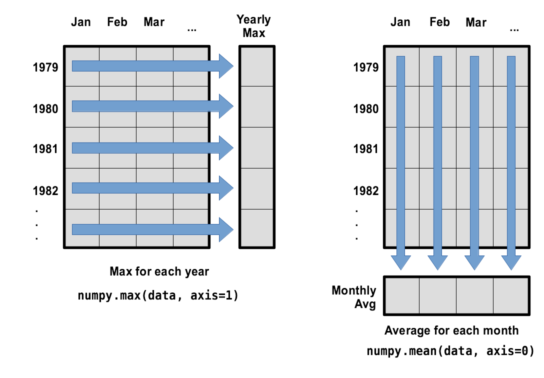
To support this functionality, most array functions allow us to specify the axis we want to work on. If we ask for the average across axis 0 (rows in our 2D example), we get:

PYTHON

print(numpy.mean(reshaped_data, axis=0))

OUTPUT

[4.59956757 4.39708108 4.09156757 3.26016216 2.60437838 2.3072973
 2.18940541 2.32145946 2.9907027  3.55627027 3.90345946 4.38140541]

As a quick check, we can ask this array what its shape is:

PYTHON

print(numpy.mean(reshaped_data, axis=0).shape)

OUTPUT

(12,)

The expression (12,) tells us we have an N×1 vector, so this is the average wave height per month for all years. If we average across axis 1 (columns in our 2D example), we get:

PYTHON

print(numpy.mean(reshaped_data, axis=1))

OUTPUT

[3.34       3.15183333 3.29866667 3.53366667 3.448      3.23016667
 2.99383333 3.51133333 2.96066667 3.20316667 3.62116667 5.1915
 3.28816667 3.529      3.523      3.66866667 3.314      2.99916667
 3.45983333 3.16783333 3.413      3.3435     3.031      3.29366667
 3.138      3.29716667 3.3185     3.24966667 3.4135     3.42866667
 3.168      2.78816667 3.61366667 3.2725     3.32766667 3.2765
 4.385     ]

which is the average wave height per month across all years.

Saving Data

---

There are occasions though the rest of the lesson when we will want to use the reshaped data. If we close this Notebook, we’ll lose the variables we’ve created, so let’s save the reshaped data to a file:

PYTHON

numpy.savetxt("reshaped_data.csv", reshaped_data, delimiter=',')

Stacking Arrays

Arrays can be concatenated and stacked on top of one another, using NumPy’s vstack and hstack functions for vertical and horizontal stacking, respectively.

PYTHON

A = numpy.array([[1,2,3], [4,5,6], [7, 8, 9]])
print('A = ')
print(A)
>
B = numpy.hstack([A, A])
print('B = ')
print(B)
>
C = numpy.vstack([A, A])
print('C = ')
print(C)

OUTPUT

A =
[[1 2 3]
 [4 5 6]
 [7 8 9]]
B =
[[1 2 3 1 2 3]
 [4 5 6 4 5 6]
 [7 8 9 7 8 9]]
C =
[[1 2 3]
 [4 5 6]
 [7 8 9]
 [1 2 3]
 [4 5 6]
 [7 8 9]]

Write some additional code that slices the first and last columns of A, and stacks them into a 3x2 array. Make sure to print the results to verify your solution.

Show me the solution

A ‘gotcha’ with array indexing is that singleton dimensions are dropped by default. That means A[:, 0] is a one dimensional array, which won’t stack as desired. To preserve singleton dimensions, the index itself can be a slice or array. For example, A[:, :1] returns a two dimensional array with one singleton dimension (i.e. a column vector).

PYTHON

D = numpy.hstack((A[:, :1], A[:, -1:]))
print('D = ')
print(D)

OUTPUT

D =
[[1 3]
 [4 6]
 [7 9]]

Show me the solution

An alternative way to achieve the same result is to use Numpy’s delete function to remove the second column of A.

PYTHON

D = numpy.delete(A, 1, 1)
print('D = ')
print(D)

OUTPUT

D =
[[1 3]
 [4 6]
 [7 9]]

Change In Wave Height

In the wave data, one row represents a series of monthly data relating to one year. This means that the change in height over time is a meaningful concept representing seasonal changes. Let’s find out how to calculate changes in the data contained in an array with NumPy.

The numpy.diff() function takes an array and returns the differences between two successive values. Let’s use it to examine the changes each day across the first 6 months of waves in year 4 from our dataset.

PYTHON

year4 = reshaped_data[3, :]
print(year4)

OUTPUT

[3.73  4.886 4.76  3.188 2.528 1.662 1.952 2.388 3.336 4.034 4.502 5.438]

Calling numpy.diff(year4) would do the following calculations

OUTPUT

[ 4.886 - 3.73, 4.76 - 4.886, 3.188 - 4.76, 2.528 - 3.188, 1.662 - 2.528, 1.952 - 1.662, 2.388 - 1.952, 3.336 - 2.388, 4.034 - 3.336, 4.502 - 4.034, 5.438 - 4.502 ]

and return the 11 difference values in a new array.

PYTHON

numpy.diff(year4)

OUTPUT

[ 1.156 -0.126 -1.572 -0.66  -0.866  0.29   0.436  0.948  0.698  0.468
 0.936]

Note that the array of differences is shorter by one element (length 11). Where we see a negative change in wave height, it shows that the sea is becoming calmer as we move towards the summer. Positive wave heights in the autumn show waves are increasing.

If the shape of an individual data file is (60, 40) (60 rows and 40 columns), what would the shape of the array be after you run the diff() function and why?

Show me the solution

The shape will be (60, 39) because there is one fewer difference between columns than there are columns in the data. {: .solution}

How would you find the largest change in wave height from month to month within each year? What does it mean if the change in height is an increase or a decrease?

Show me the solution

By using the numpy.max() function after you apply the numpy.diff() function, you will get the largest difference between months.

PYTHON

numpy.max(numpy.diff(reshaped_data, axis=1), axis=1)

OUTPUT

array([1.086, 1.806, 1.776, 1.156, 1.692, 1.274, 0.798, 2.59 , 1.338,
      1.634, 0.992, 0.618, 1.054, 1.652, 1.472, 1.716, 0.766, 1.496,
      1.656, 1.04 , 1.228, 1.336, 1.564, 1.066, 1.242, 1.604, 0.802,
      1.04 , 0.652, 0.86 , 1.176, 0.97 , 1.68 , 1.556, 1.904, 2.936,
      1.578])

If wave height values decrease along an axis, then the difference from one element to the next will be negative. If you are interested in the magnitude of the change and not the direction, the numpy.absolute() function will provide that.

Notice the difference if you get the largest absolute difference between readings.

PYTHON

numpy.max(numpy.absolute(numpy.diff(reshaped_data, axis=1)), axis=1)

OUTPUT

array([1.956, 1.806, 1.776, 1.572, 3.6  , 2.418, 0.954, 2.798, 1.338,
       1.634, 2.13 , 0.93 , 1.054, 1.71 , 1.68 , 2.   , 1.614, 1.496,
       2.308, 1.04 , 2.014, 1.68 , 1.564, 1.596, 1.528, 1.604, 1.468,
       1.21 , 1.012, 0.86 , 1.732, 1.03 , 1.68 , 1.774, 1.904, 2.936,
       1.694])

Key Points

• “Import a library into a program using import libraryname.”
• “Use the numpy library to work with arrays in Python.”
• “The expression array.shape gives the shape of an array.”
• “Use array[x, y] to select a single element from a 2D array.”
• “Array indices start at 0, not 1.”
• “Use low:high to specify a slice that includes the indices from low to high-1.”
• “Use # some kind of explanation to add comments to programs.”
• “Use numpy.mean(array), numpy.max(array), and numpy.min(array) to calculate simple statistics.”
• “Use numpy.mean(array, axis=0) or numpy.mean(array, axis=1) to calculate statistics across the specified axis.”