All in One View

Content from Data Formats, Metadata, and Vocabulary

---

Last updated on 2026-08-10 | Edit this page

Overview

Questions

• “What are the main data formats used to store ocean and atmosphere data?”
• “What is metadata, and how does it help other people find and understand my data?”
• “What is a controlled vocabulary, and why is it better than free text?”
• “Which international standards should I be aware of when publishing environmental data?”
• “How do these standards connect to modern cloud‑native formats like Zarr?”

Objectives

• “Recognize common data formats used in oceanography and meteorology (e.g. NetCDF, GRIB, BUFR, Zarr).”
• “Explain what metadata is and why it is essential for discovery and reuse.”
• “Describe what controlled vocabularies are and how they support consistent metadata.”
• “Identify key international and community standards (CF conventions, ISO 19115/INSPIRE, MEDIN, NERC NVS).”
• “Relate traditional formats and standards to emerging cloud‑native formats such as Zarr.”

Why formats and metadata matter

---

When we work with environmental data, we are not just storing the data itself. We also need to encode meaning: what was measured, where, when, how, and under which conditions. Good choices of data format and metadata make this meaning accessible to both humans and machines, enabling discovery, analysis, and long‑term reuse.

Broadly:

• Formats define how data and metadata are physically organised (arrays vs tables, gridded vs vector, binary vs text, cloud‑native vs legacy).
• Metadata and vocabularies define the semantics: variable names, units, coordinate reference systems, quality information, and controlled terms.

Using standards‑aware formats together with a good metadata and controlled vocabulary helps ensure that environmental data is self‑describing and semantically consistent, which is essential for interoperability across models, archives, visualisation tools, and cloud‑native services. Following widely used standards also means we can plug into existing tools and infrastructures (catalogues, visualisation software, cloud services) instead of reinventing everything ourselves.

Common data formats in oceanography and meteorology

---

Environmental scientists use several families of formats. Here we focus on those most relevant to gridded, multidimensional ocean and atmosphere data, and then briefly note other formats that appear around them in modern workflows.

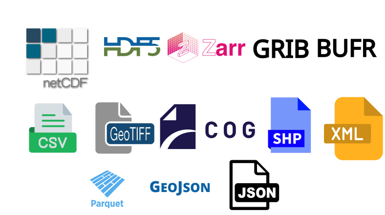
Self‑describing array formats

These formats store both array data and structural metadata (dimensions, variables, units, coordinate systems) in the same file or object:

• NetCDF (Network Common Data Form) is a machine‑independent, binary, self‑describing format designed for array‑oriented scientific data, widely used to store gridded climate, ocean and meteorological variables.
• HDF5 (Hierarchical Data Format) is another self‑describing format supporting large, complex datasets with a “directory‑like” internal structure. It is used for satellite products, model output and other multidimensional data.
• Zarr is a newer, cloud‑native format for chunked, N‑dimensional arrays. The GeoZarr standard describes how to represent geospatial datasets in Zarr using concepts from the Unidata Common Data Model, including dimensions, coordinate variables, attributes and metadata style.

This “self‑describing” property is particularly important for large climate model outputs, reanalysis products and ocean observing systems, where many different tools need to interpret the same files without bespoke documentation.

WMO exchange formats

The World Meteorological Organization maintains binary formats optimised for exchange over telecommunications networks:

• GRIB (GRIdded Binary) is a compact, self‑describing binary format for gridded meteorological fields such as numerical weather prediction (NWP) output.
• BUFR (Binary Universal Form for the Representation of meteorological data) is a flexible, table‑driven binary format designed to represent many kinds of meteorological and oceanographic observations efficiently.

These WMO “table‑driven code forms” are widely adopted for transmitting satellite products and model fields between operational centres and can also be used for storage. You will often encounter reanalysis products and forecast grids available as GRIB or NetCDF, sometimes convertible between them.

Other and emerging formats you may come across

Alongside the array formats above, you will often work with:

• ASCII / CSV: simple text tables, easy to read but not ideal for large multidimensional data.
• GeoTIFF: common in remote sensing and GIS for 2D georeferenced images such as sea‑surface temperature or altimetry maps. The Cloud‑Optimized GeoTIFF (COG) is a widely used cloud‑native variant.
• GeoJSON: a JSON‑based format for vector geometries and attributes, often used for footprints, regions of interest, and feature‑based metadata in web APIs and STAC items.
• Shapefiles: an older but still common vector format in GIS for points, lines and polygons describing stations, coastlines, regions, etc.
• Parquet / GeoParquet: columnar, compressed table formats increasingly used in cloud‑native analytics. GeoParquet adds conventions for storing vector geometries alongside tabular attributes, making large point or polygon datasets efficient to query in data lakes and lakehouses.
• XML / JSON: often used for metadata documents, catalog records or service responses, rather than bulk gridded data.

Callout

Concept: “Self‑describing” data

A file is called self‑describing when it contains enough structural metadata (dimensions, variables, units, coordinate systems) that a tool can understand and subset the data without external manuals or code lists. NetCDF, HDF5, GRIB, Zarr and CF conventions all aim to make scientific files self‑describing.

The other formats (vector, tabular, point‑cloud, XML/JSON) typically rely more on external schemas or conventions, and are often used to provide context and cataloguing around core array datasets rather than to store the primary model or reanalysis fields themselves.

Callout

Parquet and GeoParquet in practice

Parquet and GeoParquet are increasingly used as cloud‑native table and vector formats in data lakes and lakehouses, especially for large point, line and polygon datasets. They are replacing many large CSV and Shapefile/GeoJSON workflows in logistics, urban planning, mobility, environmental monitoring, remote sensing, and national‑scale GIS platforms, because they are compact, fast to scan, and integrate directly with analytics engines like Spark, DuckDB, BigQuery, Snowflake and modern GIS tools.

In this course, we mention Parquet/GeoParquet as part of the broader cloud‑native ecosystem, but our main focus is on self‑describing array formats (NetCDF, HDF5, Zarr and GeoZarr) for multidimensional ocean and atmosphere data.

What is metadata?

---

Metadata is “data about data”: information that describes a dataset so that people (and software) can understand, find, and reuse it.

In the marine and atmospheric domains, common metadata elements include:

• Who collected the data and why.
• What was measured (variables, units, methods).
• Where and when (spatial/temporal coverage, coordinate reference system).
• How it was processed (algorithms, quality flags, versions).
• How to access, cite, and interpret it.

Standards such as ISO 19115 for geographic information define sets of metadata elements covering identification, extent, quality, spatial and temporal schema, reference systems and distribution. These are used in catalogues and portals to support dataset discovery and evaluation.

Source

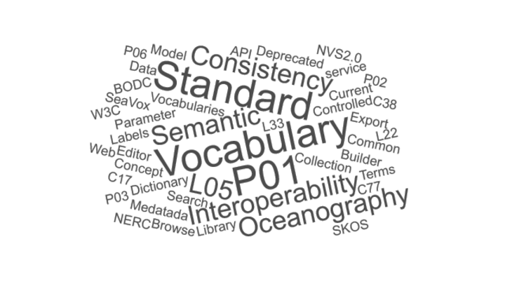
Controlled vocabularies and vocabulary services

Free‑text metadata can be ambiguous (“temp”, “T”, “temperature”) and hard to search. Controlled vocabularies fix this by providing curated lists of standard terms and identifiers.

The NERC Vocabulary Server (NVS), operated by the British Oceanographic Data Centre (BODC), publishes centrally managed lists of terms for annotating marine and related Earth science data, using the SKOS (Simple Knowledge Organization System) model to represent concepts and collections. NVS hosts vocabularies for platforms, instruments, parameters, projects, geographic regions and more. These vocabularies are used to:

• Populate drop‑down lists in metadata editors, ensuring consistent choice of parameter names, platforms, and methods.
• Mark up metadata with stable URIs rather than free text, enabling machine‑readable search and semantic cross‑walks between different metadata schemas.
• Support “smart search” and semantic web services in marine data portals, including collections specifically for MEDIN controlled vocabularies and SeaDataNet common vocabularies.

MEDIN’s Discovery Metadata Standard is a marine profile of the UK government’s GEMINI standard and is aligned with INSPIRE and ISO 19115, providing a consistent template for describing marine datasets in the UK context. This profile focuses on “discovery metadata”, the core elements needed for catalogues and portals to help users find and evaluate datasets.

Callout

Example: A parameter name from NVS

A single measured variable (e.g. “sea water temperature at 5 m”) might be described by a P01 code in NVS that encodes the phenomenon, medium, vertical position and statistical operation in a single, standardised label. Using that code in your metadata ensures different datasets use exactly the same concept when they mean the same thing.

Key standards you should know

---

CF metadata conventions

The Climate and Forecast (CF) metadata conventions define how to describe Earth science data in self‑describing formats (originally NetCDF) so that files from different sources can be processed and compared consistently. CF specifies attributes such as standard_name, units, cell_methods, coordinates, bounds and grid_mapping, plus rules for how to represent grids, time coordinates and climatological statistics.

CF has been widely adopted for atmosphere and ocean data, including climate model output for major intercomparison projects, and is considered a recommended standard for gridded data in programmes like IOOS.

ISO 19115, INSPIRE, and profiles

ISO 19115 is the international standard for describing geographic information and services, covering identification, extent, quality, spatial/temporal schema, spatial reference and distribution. The INSPIRE Metadata Implementing Rules define how to implement discovery metadata using ISO 19115 and related standards for spatial data sets and services in the European context.

MEDIN’s Discovery Metadata Standard is an ISO 19115‑based UK profile, ensuring that marine metadata records are compliant with INSPIRE and ISO while tailored to national practice. Other marine communities, such as SeaDataNet, also use ISO 19115‑based community profiles for their portals.

WMO code forms and operational formats

The WMO maintains binary and alphanumeric code forms such as BUFR and GRIB for efficient exchange of meteorological and oceanographic data over telecommunication networks. GRIB is widely used for NWP output, while BUFR is used for high‑volume observational data (satellites, aircraft reports, profilers) and can include quality information alongside the observations.

Operational data centres and services often distribute ocean and marine meteorological data in formats such as NetCDF, GRIB and BUFR, which are recognised by cloud platforms and big‑data tools.

STAC - SpatioTemporal Asset Catalogs

STAC (SpatioTemporal Asset Catalogs) defines a common JSON/GeoJSON‑based language to describe and organise geospatial assets (files, APIs, data cubes) in space and time. It introduces three core objects:

• Catalog: an entry point that links to Collections and Items.
• Collection: a grouped set of related data (e.g. “ERA5 surface climate cubes”), with shared metadata and spatial/temporal extent.
• Item: a single spatiotemporal asset (e.g. one product or one NetCDF file), linking to the actual data files via “assets”.

STAC is often used on top of ISO 19115‑style discovery metadata: ISO profiles provide rich descriptions, while STAC standardises how those assets are organised and queried via static catalogs or STAC APIs. In this course we focus mainly on CF and NVS for internal metadata, but later lessons show how STAC can reference datasets and support cloud‑native discovery workflows.

Metadata inside data files vs discovery metadata

In formats like NetCDF, metadata lives “inside” the file as attributes attached to variables and dimensions (e.g. units, standard_name, long_name, history). Normally, this metadata is structured according to the CF conventions, which allow software tools to interpret the data correctly.

Discovery metadata standards (MEDIN, GEMINI, INSPIRE, ISO 19115, STAC) describe datasets at a higher level, typically as XML or JSON records in catalogues, including title, abstract, keywords, contact, spatial/temporal extent, and links to data services.

Both layers are needed: internal metadata lets analysis tools interpret arrays correctly, while discovery metadata lets users and catalogues know the dataset exists and decide whether it is suitable for their purpose.

Challenge

Exercise 1 - Match format and standard

For each scenario, suggest a “format + metadata standard” combination that would be appropriate, and explain your reasoning.

1. Global daily sea surface temperature reanalysis on a regular grid, published for long‑term reuse.
2. Ship‑based CTD profiles with detailed instrument metadata, to be ingested into a national marine data centre.
3. Operational global numerical weather prediction forecast fields disseminated to weather services every 6 hours.

Take 5 minutes to think or discuss in pairs, then share your answers.

Show me the solution

Example answers:

1. NetCDF (or cloud‑native Zarr) with CF conventions for internal metadata, plus an ISO 19115/INSPIRE‑compliant discovery metadata record using the relevant national profile (e.g. MEDIN Discovery Metadata in the UK), and a STAC Collection/Items to expose the Zarr stores in a cloud‑native catalog.
2. NetCDF or CSV for the data, with rich internal metadata (units, calibration info) and discovery metadata following MEDIN Data Guidelines and Discovery Metadata Standard, using NVS controlled vocabularies for parameters, platforms and instruments, and optionally STAC Items to reference individual cruises or deployments.
3. GRIB (or GRIB2) as the WMO‑recommended binary format for gridded NWP forecasts, with WMO‑compliant GRIB metadata, and catalogue / API metadata using ISO 19115/INSPIRE or the relevant organisational profile, potentially wrapped in a STAC Collection and Items for each forecast run to support cloud‑native discovery.

Why following standards is so important

---

Using community standards has practical benefits:

• Interoperability: CF‑compliant NetCDF datasets can be read by widely used libraries (xarray, Iris, CF‑Python), visualisation tools and data portals without custom code.
• Discoverability: ISO 19115 / INSPIRE / MEDIN‑compliant metadata records can be harvested by catalogues, making your data visible in national and international portals.
• Semantic clarity: Controlled vocabularies via NVS ensure that different datasets and organisations use the same, well‑defined concepts for parameters, platforms and methods, reducing ambiguity.
• Governance and efficiency: Embedding data management (including standards, metadata and vocabularies) into organisational policy can reduce risk, support audits, and lower costs over the data lifecycle.

For cloud‑native data, standards are what allow us to move from traditional files to object storage and APIs without losing meaning: GeoZarr’s alignment with CF and NetCDF, and catalogue metadata aligned with STAC, make Zarr‑based datasets interoperable with both scientific and geospatial ecosystems.

Challenge

Exercise 2 - Spot the missing metadata

Imagine you find a file sst_daily.nc containing a global sea surface temperature field. Inside the file you see:

• Variable name: temp
• No units attribute
• No standard_name attribute
• Time coordinate has values but no calendar or reference time (e.g. “days since …”)

Discuss:

1. What problems might this cause for someone else trying to use the data?
2. Which CF and/or ISO/MEDIN metadata elements would you add to improve the situation?

Take 5 minutes, then share your ideas.

Show me the solution

Example answers:

1. Without units, users cannot be sure whether temp is in Kelvin, Celsius, or something else. Without standard_name, automated tools cannot recognise the variable as sea surface temperature. Ambiguous time coordinates make it hard to align with other datasets or interpret the temporal coverage.
2. At minimum, add CF attributes: standard_name="sea_surface_temperature", units="K" (or appropriate units), long_name describing the variable, and proper time metadata (e.g. time with units="days since 1970-01-01" and calendar="gregorian"), plus a descriptive title and institution for provenance. In discovery metadata (ISO 19115 / MEDIN), ensure fields like abstract, keywords (from NVS vocabularies), temporal extent and geographic bounding box are populated.

Key Points

• “Oceanography and meteorology rely on self‑describing array formats (NetCDF, HDF5, Zarr) and WMO exchange formats (GRIB, BUFR) for gridded and observational data.”
• “Metadata is ‘data about data’ and lives both inside files (e.g. CF attributes) and in separate discovery records based on standards such as ISO 19115, INSPIRE and MEDIN.”
• “Controlled vocabularies, delivered through services like the NERC Vocabulary Server, provide standardised terms and identifiers that make metadata consistent and machine‑actionable.”
• “CF metadata conventions define how to describe Earth science variables, grids and coordinates in self‑describing formats and underpin many ocean and climate data tools.”
• “Discovery profiles such as the MEDIN Discovery Metadata Standard align national practice with international standards (ISO 19115, INSPIRE), supporting data discovery across portals and organisations.”
• “STAC catalogs (Catalogs, Collections, Items) provide a modern, JSON‑based way to organise and expose geospatial assets, including NetCDF and Zarr stores, in cloud‑native workflows.”
• “Cloud‑native formats like Zarr become interoperable when combined with established metadata and vocabulary standards (CF, Unidata CDM, ISO profiles, NVS) and can be complemented by STAC for discovery.”

Content from Challenges of N-Dimensional Data

---

Last updated on 2026-08-05 | Edit this page

Overview

Questions

• “How do NetCDF, GRIB, and HDF5 organise large n-dimensional arrays?”
• “Why have typical datasets in meteorology and oceanography grown so much in size?”
• “What happens when we open these files in standard tools like xarray?”
• “Why is it important to share data in a way that supports partial access rather than whole-file downloads?”
• “How do chunking and parallel processing affect performance, scalability, and memory use?”

Objectives

• “Describe how NetCDF, GRIB, and HDF5 organise n-dimensional data and impact file size.”
• “Explain why meteorological and oceanographic datasets have grown so large over the last 30 years.”
• “Recognise practical challenges when opening, sharing, and inspecting NetCDF and GRIB files.”
• “Explain why we do not want to download whole files all the time, and how partial access and chunking help.”
• “Gain hands-on experience exploring file structure and chunks with xarray as a first step toward cloud-native solutions.”

Why n-dimensional data is hard

---

In oceanography and meteorology, most core data products are naturally n-dimensional: time, latitude, longitude, height or depth, and often additional dimensions such as ensemble member, forecast lead time, and variable.

Source

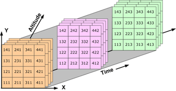
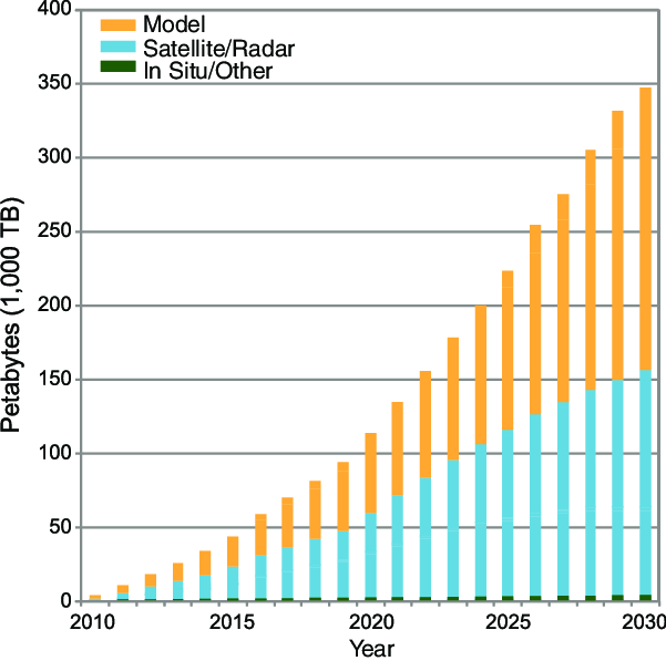
Over the last three decades, higher spatial and temporal resolution, more vertical levels, longer archives, and ensembles have pushed typical file sizes from megabytes to gigabytes, and today large collections can reach terabytes or petabytes.

Early attempts to manage this data with generic database systems ran into limitations: they did not treat multidimensional arrays as first-class objects and performed poorly on large scientific datasets, motivating specialised formats like NetCDF and GRIB.

NetCDF: self-describing arrays

NetCDF was designed in the late 1980s as a portable, self-describing file format and data model for array-oriented scientific data such as climate and ocean model output. A NetCDF file stores variables (arrays), dimensions (e.g. time, lat, lon, level), and attributes (metadata) in a single container, enabling programs to discover structure and metadata at runtime without relying on separate documentation.

NetCDF-3 stores data in a simple, contiguous layout, while NetCDF-4 builds on HDF5 as a storage layer, adding features such as groups and support for very large arrays and complex hierarchies. From the user’s point of view, NetCDF provides an intuitive way to represent n-dimensional fields. But as datasets grow, organisational choices (e.g. which dimensions to include, how to structure variables and files) strongly affect how easy they are to work with.

GRIB: compact operational exchange

GRIB (GRIdded Binary) is a World Meteorological Organization format designed for efficient transmission and storage of gridded meteorological fields, especially numerical weather prediction outputs. It uses many “messages”, each containing a field plus encoded metadata, and is governed by WMO tables that define parameters, levels, and other descriptors.

GRIB was declared operational as a standard in the early 2000s with GRIB2, providing more flexible metadata, additional compression methods, and improved support for missing values compared to the original GRIB. This message-based structure is highly compact and well suited to operational workflows, but it can be more difficult to treat GRIB files as simple n-dimensional arrays, and heterogeneous messages may need to be filtered or regrouped before analysis.

HDF5: a general high-performance container

HDF5 is a general hierarchical data format that supports large, complex datasets, and underpins NetCDF-4’s storage layer. It provides groups, datasets, and rich metadata, allowing complex scientific data structures to be represented in a single file, and has been widely adopted beyond atmospheric science, including in remote sensing and other Earth-observation products.

NetCDF-4 hides much of HDF5’s complexity behind the NetCDF API and data model, so most users interact with variables, dimensions, and attributes rather than low-level storage details. However, the ability to represent large hierarchical datasets efficiently is one reason NetCDF-4/HDF5 has become a backbone for many modern environmental archives.

Thirty years of growing data volumes

Over roughly the last 30 years, several trends have driven data growth in meteorology and oceanography:

• Higher spatial resolution in models and reanalyses, moving from coarse global grids to kilometre-scale domains.
• Higher temporal resolution, with more frequent output (e.g. hourly, sub-hourly) instead of monthly or daily only.
• More vertical levels in atmosphere and ocean models, capturing detailed vertical structure.
• Longer archives of observations and reanalyses, often spanning many decades.
• Ensembles of forecasts and climate simulations, multiplying data volume by the number of members.

These trends have pushed archives from simple files to huge collections, requiring careful selection of formats, file organisation strategies, and access tools.

The volume of worldwide climate data is expanding rapidly ¹

Typical access patterns today

---

In many workflows, meteorology and oceanography practitioners:

• Use NetCDF (NetCDF-3 or NetCDF-4/HDF5) for archival and analysis of gridded fields and time series.
• Use GRIB for operational forecast products and exchange between centres.
• Rely on high-level libraries such as xarray to open NetCDF and GRIB files and represent them as labelled n-dimensional datasets.

From the perspective of “The NetCDF Developer’s Handbook”², high-performance programs must understand both the logical data model (variables, dimensions, attributes) and practical constraints (file size, number of files, hardware) to manage scientific data effectively. This episode focuses on understanding the problem space and the structures we are working with.

Challenge

Exercise 1: Inspecting the structure of a NetCDF file

The example NetCDF file data/era5_sst/ocean_temperature.nc contains a subset of the ERA5 Reanalysis, consisting of 2D sea surface temperature fields (latitude and longitude) recorded every 2 hours during the first five days of 2025.

1. Use xarray to open the dataset.
2. Inspect dimensions, coordinates, and attributes.
3. Discuss how the organisation (variables, dimensions, attributes) reflects the n-dimensional nature of the data.

PYTHON

import xarray as xr

base_path = "/gws/ssde/j25b/atlantis_vis/cloud-native-geoscience-course/" # or "" if you have the data in your current working directory

ds = xr.open_dataset(f"{base_path}data/era5_sst/ocean_temperature.nc")
print(ds)
print(ds.dims)
print(ds.coords)
print(ds.attrs)

Think about:

• Which dimensions does this dataset use (e.g. time, lat, lon, depth)?
• How would the structure change if we added ensemble members or vertical levels?
• What might become difficult as the dataset grows larger or more complex?

Show me the solution

This dataset has dimensions for “time” (valid_time), “lat” (latitude), and “lon” (longitude), with corresponding coordinate variables. Attributes provide metadata about the dataset, such as the source, institution, and conventions used. Adding ensemble members or more levels would introduce additional dimensions, increasing the size of the dataset and potentially complicating access patterns.

Challenge

Exercise 2 - Comparing NetCDF and GRIB files

Many forecast products are distributed in GRIB, while climate or reanalysis products may be available as NetCDF. To get a feeling for differences:

1. Open a NetCDF example (e.g. data/era5_sst/ocean_temperature.nc) with xarray.
2. Open a GRIB example (e.g. data/era5_sst/ocean_temperature.grib) with xarray using the cfgrib engine.
3. Compare what print(ds) shows for each: dimensions, data variables, coordinates, and attributes.

To open a GRIB file, you may need to use engine="cfgrib" in xr.open_dataset():

PYTHON

ds_grib = xr.open_dataset(
    f"{base_path}data/era5_sst/ocean_temperature.grib",
    engine="cfgrib",
)
print(ds_grib)
print(ds_grib.dims)
print(ds_grib.data_vars)

Questions to discuss:

• Do both files present regular grids with similar dimensions (e.g. latitude, longitude, time)?
• How many variables are present in each, and how are they named?
• What metadata is available (e.g. attributes for conventions, originating centre, parameter names)?

Show me the solution

Both files expose a very similar data model when opened with xarray. They contain the same spatial grid (721 × 1440), 120 time steps, and a single variable (sst). The main difference is in the temporal and auxiliary coordinates: the NetCDF file uses valid_time as its dimension, whereas the GRIB file uses time as the dimension and retains additional GRIB-specific coordinates such as step, surface, and number. The GRIB dataset also preserves extra metadata, such as the GRIB edition, while the NetCDF file presents a simplified CF-compliant representation. In general, NetCDF stores dimensions, variables, and metadata explicitly, whereas GRIB is a message-based format where much of the metadata is encoded within each field.

Challenge

Exercise 3 - Thinking about growth and organisation

Using the data/era5_sst/ocean_temperature.nc NetCDF file, imagine that:

• Spatial resolution doubles in each horizontal direction.
• Output frequency increases from monthly to hourly.
• We add more time steps to cover a 30‑year period.
• Several colleagues also need to analyse this dataset, possibly from different institutions.

Discuss:

1. How would this change the dimensions of your dataset (e.g. lat, lon, time, depth)?
2. How might file sizes change for a single file and for the full archive?
3. What practical challenges might you face when trying to open and inspect such datasets with the same tools?
4. How would you share this growing dataset today (local copies, shared server, remote service), and what problems might that create?

You do not need to implement anything. Focus on reasoning about dimensions, size, organisation, and sharing.

Show me the solution

Doubling the horizontal resolution would increase the number of latitude and longitude points, giving about four times more grid cells at each time step. Changing the output from monthly to hourly and extending the dataset to 30 years would greatly increase the number of time steps, making the dataset much larger overall.

A single file would become difficult to store, move, and analyse, so it would be better to split the data into smaller files. Opening and working with the full dataset would also become slower and could require more memory than is available on a typical computer.

Sharing the dataset by giving everyone a local copy would be inefficient because of its size and could lead to different versions of the data. A better option would be to store the dataset on a shared server or in cloud storage, so everyone can access the same data without downloading the entire archive.

Sharing data and accessing subsets

---

As data volumes grow, the way we share and access n-dimensional datasets becomes just as important as the way we store them.

Traditional patterns: download first, analyse later

In many workflows, people still:

• Publish NetCDF or GRIB files on an FTP/HTTP server or data portal.
• Download complete files to local disk or a shared server.
• Open them with tools like xarray or command‑line utilities.

For small datasets this is fine, but for multi‑gigabyte or multi‑terabyte archives it is neither efficient nor scalable:

• Whole‑file downloads are slow and expensive (network, storage, time).
• Users often need only a subset (e.g. one variable, a region, a time window), not the full archive.
• Multiple users pulling the same large files creates unnecessary duplication and storage overhead.

Even when chunking is used inside NetCDF‑4/HDF5, the file is still treated as a single object: clients ultimately have to read data from that file (locally or via a server) to do any calculation, and classical NetCDF/HDF5 are optimised for POSIX‑style file systems rather than direct object‑store access.

Callout

POSIX file systems and object storage

A POSIX file system is a traditional file-system model with directories, files, and paths that are accessed through a local or mounted storage interface. It is commonly used for shared filesystems and local disks.

An object-store file system is a storage interface that exposes object storage through filesystem-like operations, often used in cloud workflows. It is different from a traditional POSIX filesystem because data are accessed through object APIs rather than a normal directory tree.

Server‑side subsetting and remote access

Server‑side access protocols such as OPeNDAP and modern APIs allow clients to request subsets of NetCDF data (e.g. a bounding box in space and a time range) without transferring the entire file, which is already a step toward “not download the whole file all the time”. These services can reduce duplication and help centralise access, but they require maintained infrastructure, and performance still depends on server load and network bandwidth.

Storage considerations

Storing large archives on traditional networked file systems or shared servers can become costly and hard to scale, especially when data are kept online for many years. Cloud and institutional infrastructures increasingly use object storage for large, mostly read‑only datasets, because it scales horizontally and can be cheaper per terabyte for large volumes of unstructured scientific data.

In this lesson we do not go into technical details of object stores or cloud pricing, but it is useful to recognise that:

• Growing data volumes make it expensive to keep multiple full copies on local disks or HPC filesystems.
• Centralised archives and object storage are attractive for long‑term, shared access.
• Formats and access patterns that support subsetting and streaming (rather than whole‑file downloads) will become more important as archives grow.

Later lessons on Zarr and cloud‑native workflows will show how chunking, object storage, and tools like xarray/dask are combined to address these challenges more directly.

Callout

A note on access and storage

NetCDF and GRIB are often used in a “download first, analyse later” workflow, where people copy the whole file to a local machine or shared server before opening it. Xarray can be lazy when it opens NetCDF files, so metadata can be inspected without immediately reading all values, but many analyses still end up pulling large parts of the file into memory when the data are actually used. In practice, this means that sharing data efficiently is still a challenge, especially when many people need access to the same large archive.

For that reason, large scientific archives are often easier to manage on central servers or object storage systems than as many duplicated local copies. Classical NetCDF/HDF5 workflows also tend to fit better with shared file systems than with direct object storage, which is one reason cloud-native formats such as Zarr are becoming important later in this course.

Summary: format, scale, and access as core challenges

---

Over the last 30 years, meteorology and oceanography have moved from modest, locally processed datasets to global, multi‑decadal archives and high‑resolution forecasts stored in specialised formats. NetCDF (particularly NetCDF‑4/HDF5) provides a flexible, self‑describing model for n‑dimensional arrays that has become central to many scientific archives, while GRIB offers compact, operational‑oriented storage and transmission for gridded meteorological fields governed by WMO codes and tables.

Today, tools such as xarray allow us to open both NetCDF and GRIB as labelled n‑dimensional datasets, but the growing scale of data and the organisational choices made in these formats create real challenges for sharing data efficiently, avoiding whole‑file downloads, and managing performance, scalability, memory, and storage cost. Server‑side subsetting and chunked storage help, but classical file‑based formats are still built around single files and shared file systems. The rest of the course will show how cloud‑native formats and workflows build on these ideas, especially chunking and object storage, to make large n‑dimensional data more manageable.

Key Points

• “NetCDF provides a self‑describing, array‑oriented data model for n‑dimensional scientific datasets and is widely used in meteorology and oceanography.”
• “GRIB is a compact, message‑based WMO format designed for operational transmission of gridded meteorological fields, using tables and codes to represent metadata.”
• “Data volumes have grown dramatically with higher resolution, more frequent output, longer archives, and ensembles over the last three decades.”
• “In many current workflows, large NetCDF and GRIB files are still downloaded in full to local or shared servers, even when only subsets are needed.”
• “Server‑side subsetting (e.g. OPeNDAP) and centralised archives can reduce duplication, but long‑term storage on traditional file systems becomes costly at scale compared to object storage.”
• “Understanding how existing formats organise n‑dimensional data, and where they strain under growth in size and shared use, prepares us to learn about chunking and cloud‑native solutions in later lessons.”

---

1. Overpeck, J., Meehl, G., Bony, S., & Easterling, D. (2011). Climate Data Challenges in the 21st Century. Science, 331(6018), 700-702. https://doi.org/10.1126/science.1197869↩︎

2. Harnett, E. (2026). The NetCDF Developer’s Handbook: The Authoritative Guide to Writing High-Performance Programs for Scientific Data Management.↩︎

Content from Cloud-Native Formats

---

Last updated on 2026-08-05 | Edit this page

Overview

Questions

• “What makes a format cloud-native?”
• “Why are traditional file-based formats not always a good fit for cloud storage?”
• “Which cloud-native or cloud-optimized approaches are relevant for Earth system data?”
• “How do cloud-native formats change the way we work with environmental data?”

Objectives

• “Explain what is meant by a cloud-native data format.”
• “Describe why traditional file-based formats can be inefficient in cloud environments.”
• “Identify cloud-native and cloud-optimized approaches used for environmental data, including Zarr, Kerchunk, VirtualiZarr, GeoParquet, and FlatGeobuf.”
• “Recognise why cloud-native formats matter for scalable access, sharing, and analysis.”

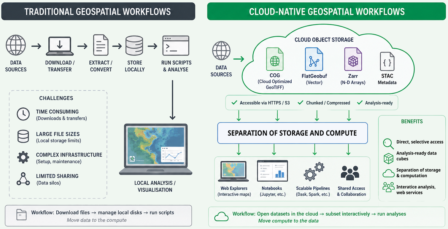
“Hey, let’s not download the whole file every time.”¹

---

Environmental data is growing rapidly in size and complexity, and traditional approaches based on downloading files are becoming increasingly impractical for scientific work. Users often cannot reasonably wait to download, store, and process very large files locally, especially when they only need a subset of the data.

Cloud-native and cloud-optimized formats aim to support more direct access to the parts of a dataset we actually need, without requiring complete file downloads first. This matters in oceanography, climate, and meteorology, where datasets are often large, multidimensional, and shared by many users.

From files to cloud objects

Traditional scientific formats such as NetCDF, GRIB, and HDF5 were designed mainly for file-based storage systems: local disks, shared servers, and HPC filesystems. In that world, the standard workflow is often “download the file, open the file, analyse the file”.

Cloud storage works differently. Instead of one large file on a filesystem, data is commonly stored as many independent objects accessed over HTTP or S3-style APIs. In this setting, performance depends not just on how data is encoded, but also on how many requests are needed, where metadata lives, and whether small subsets can be fetched efficiently.

What makes a format cloud-native?

A useful community description from the Cloud-Native Geospatial Formats Guide² is that cloud-optimized formats follow a common pattern:

• Metadata provides addresses for data blocks.
• Metadata is stored in a consistent format and location.
• All metadata can be loaded with a small number of reads, ideally one.
• Libraries can use that metadata to read only the required subset of the underlying data.

For multidimensional environmental data, this usually means chunked arrays, lightweight metadata access, and layouts that work well with object storage rather than assuming a POSIX filesystem. The goal is not to change the meaning of the data, but to change how efficiently we can discover, access, and process it.

Difference between traditional files and cloud-native objects

Caution

Cloud-native does not just mean “stored in the cloud”

Putting NetCDF or HDF5 files into a cloud bucket does not automatically make them cloud-native. A format or layout becomes cloud-native or cloud-optimized when it supports efficient remote access to metadata and subsets, instead of treating cloud storage as if it were just another disk.

Key formats and approaches in Earth science

---

There is no single cloud-native solution for all environmental data, and the community guide explicitly notes that there is no one-size-fits-all approach. Instead, several complementary approaches are used.

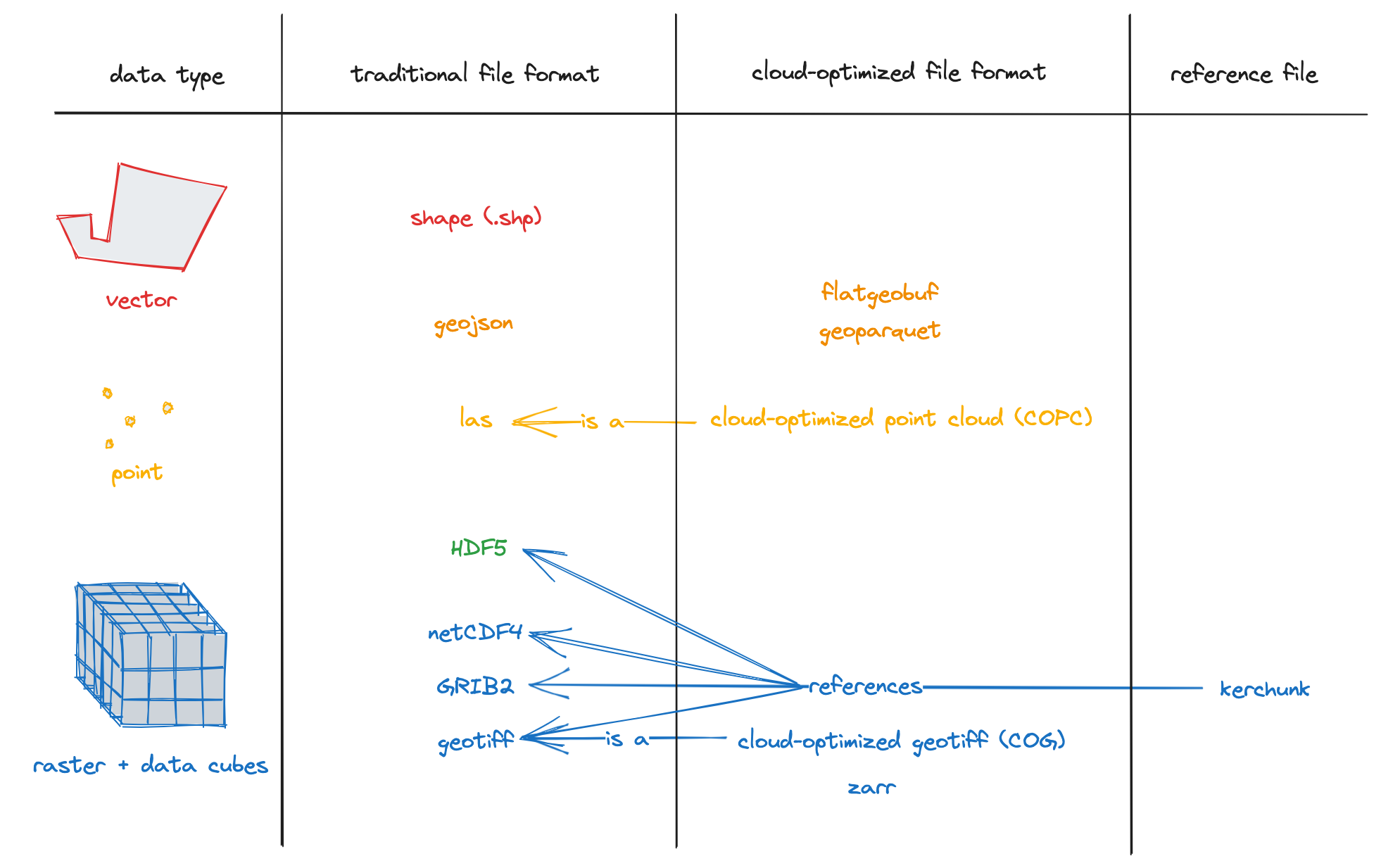
• Zarr: a format for chunked N-dimensional arrays stored as key-value objects, widely used for climate and Earth observation data.
• Kerchunk: a Python library that builds reference files describing how to read existing NetCDF/HDF5/GRIB data as if it were a Zarr store, without rewriting the original data.
• VirtualiZarr: a project for creating cloud-optimized virtual Zarr stores from existing scientific data, exposing non-Zarr data through a Zarr-like interface.
• Cloud-optimized Geotiff (COG): a format for geospatial raster data that allows efficient access to subsets of large images over HTTP or Object Storage, using internal tiling and metadata.
• GeoParquet: a cloud-friendly columnar format for geospatial vector data, built on Apache Parquet.
• FlatGeobuf: a binary geospatial vector format designed for efficient streaming and spatially indexed access, including over HTTP range requests.

In practice, these approaches support different needs. Some workflows rewrite data into a new cloud-native layout such as Zarr, while others keep legacy files and expose them through references for cloud-friendly access.

Source

Why not rely only on traditional formats?

---

Traditional formats remain essential in Earth system science, and they are not going away. However, large collections of NetCDF, HDF5, or GRIB files can be awkward in cloud environments because metadata may be embedded inside many separate files, file access patterns may generate many remote reads, and workflows often still assume that files are downloaded or mounted before analysis.

Cloud-native approaches try to reduce those problems by making metadata easier to access, enabling more selective reads, and supporting shared access from central object storage. This is especially useful when many users want small subsets of very large archives, such as time series at one point, one variable over a region, or a slice from a global model output.

How this changes workflows

---

With cloud-native approaches, the workflow can shift from “download first, analyse later” to “open remotely, inspect metadata, and read only the needed chunks”. This can reduce waiting time, duplicate local copies, and the amount of data transferred over the network.

It also supports more scalable shared analysis: the data can stay in central storage while many users, notebooks, or processing jobs access different parts of it at the same time. For this course, the most important next step is Zarr, because it gives a concrete example of how chunked, multidimensional environmental data can be organised for this style of access.

How cloud-native formats change data interaction

---

Cloud-native formats change how scientists and tools interact with environmental data:

• Direct, selective access from the cloud: users can open datasets directly over HTTPS or S3 without prior download, reading only the chunks needed for a computation or visualisation.
• Analysis-ready data cubes: archives can be restructured into large, coherent data cubes (e.g. global climate fields in Zarr with CF conventions) that are easier to query and subset across space, time, and variables.
• Separation of storage and computation: compute runs in scalable cloud environments (e.g. Kubernetes clusters, serverless platforms) while data stays in object storage, reducing data movement and enabling shared access.

In oceanography and meteorology, this means workflows can shift from “download files, manage local disks, run scripts” to “open datasets in the cloud, subset interactively, and run analyses without moving entire archives”. It also enables new services: web-based explorers, interactive notebooks, and scalable processing pipelines that operate directly on cloud-native stores, as demonstrated in several tutorials that use ERA5 data in Zarr together with STAC metadata.

Challenge

Exercise 1 - Spot the cloud-native opportunity

Think about a dataset you use in your own work, such as a reanalysis product, climate model output, or an ocean observing dataset.

Discuss:

1. How do you currently access it: download files, mount shared storage, query a service, or something else?
2. When you analyse it, do you usually need the whole dataset or only a subset?
3. What problems would be easier to solve if you could inspect metadata quickly and read only the parts you need?

Write down one example operation, such as: - extracting a time series at one point, - selecting one variable for one month, - computing a statistic over one region.

Then describe how that task might change if the dataset were available in a cloud-native form.

Show me the solution

There is no single correct answer, but many datasets are still accessed by downloading files or reading them from shared storage, even when only a small part of the data is needed.

For example, if you only want to extract sea surface temperature for one location over one month, you may still need to open a very large file. With a cloud-native dataset, you could first inspect the metadata, then read only the variable, time period, and region you need. This reduces data transfer, speeds up analysis, and allows multiple users to work from the same shared dataset without creating many local copies.

Challenge

Exercise 2 - Thinking in chunks

One of the main ideas behind Zarr is that data is divided into many smaller chunks. Instead of reading an entire dataset, software can load only the chunks needed for a particular operation.

Now, imagine a global sea surface temperature dataset stored as a Zarr archive.

For each task below, discuss which part of the dataset you would expect to read:

1. Plot sea surface temperature for one day over the whole world.
2. Extract a 10-year time series at one location.
3. Compute the average temperature over the North Atlantic for one month.

Questions:

• Would you expect to read the whole dataset or only part of it?
• Why is it useful for the data to be stored in chunks instead of one large file?
• How might the choice of chunk layout affect the speed of these different tasks?

Show me the solution

For example:

• A global map for one day mainly needs chunks covering that single time step.
• A time series at one location mainly needs chunks containing that location through time.
• A regional average only needs chunks covering the selected region and time period.

Different analyses benefit from different chunk layouts, so choosing an appropriate chunking strategy is an important part of working with Zarr datasets.

Key Points

• “Cloud-native formats are designed for efficient access over object storage and web protocols, not just for local filesystems.”
• “A cloud-native layout usually combines lightweight metadata with addressable chunks so that tools can read only the data they need.”
• “Simply storing NetCDF or HDF5 files in the cloud does not automatically make them cloud-native.”
• “In Earth system science, common approaches include Zarr, cloud-optimized NetCDF/HDF5 layouts, Kerchunk, VirtualiZarr, GeoParquet, and FlatGeobuf.”
• “Cloud-native approaches can reduce data movement, improve sharing, and support scalable analysis of large environmental datasets.”

---

1. Cheipesh, E. 2018. Available at: https://pt.slideshare.net/slideshow/cloud-optimized-geottiffs-enabling-efficient-cloud-workflows/97510557↩︎

2. Cloud-Native Geospatial Formats Guide. Available at: https://guide.cloudnativegeo.org/↩︎

Content from Zarr Data Model and Chunked Storage

---

Last updated on 2026-08-14 | Edit this page

Overview

Questions

• “What is Zarr, and how does its data model differ from formats like NetCDF or HDF5?”
• “How does Zarr store metadata about arrays and groups?”
• “What is chunked storage in Zarr, and why is it useful for large multidimensional datasets?”
• “How is Zarr changing the way ocean, climate, and meteorological data are stored and accessed?”

Objectives

• “Explain Zarr’s core data model: groups, arrays, stores, and chunks.”
• “Describe how Zarr metadata works and how conventions build on it.”
• “Understand Zarr’s chunked storage and why it matters for oceanography, climate, and meteorology.”
• “Practice opening a Zarr store with Python and xarray to see the structure in practice.”

Zarr in context

---

Zarr is an open-source format and data model for storing chunked, N-dimensional arrays in a way that works naturally with cloud object storage and file systems. It was originally developed in the scientific Python community, and has since grown into a multi-language ecosystem with implementations in Python, Rust, Julia, Matlab, R (programing language), JavaScript and others. In the Zarr website and documentation, you can find a list of implementations.

For Earth and climate data, Zarr is being adopted by major providers (e.g. ESA’s Sentinel products and National Weather Service-USA) and projects such as Earth Data Hub, Pangeo, and DestinE, precisely because it scales to petabyte-sized datasets while remaining accessible from tools like xarray.

Zarr as a data model

---

At a high level, Zarr is a way to represent large N-dimensional arrays as smaller pieces that can be stored and accessed efficiently.

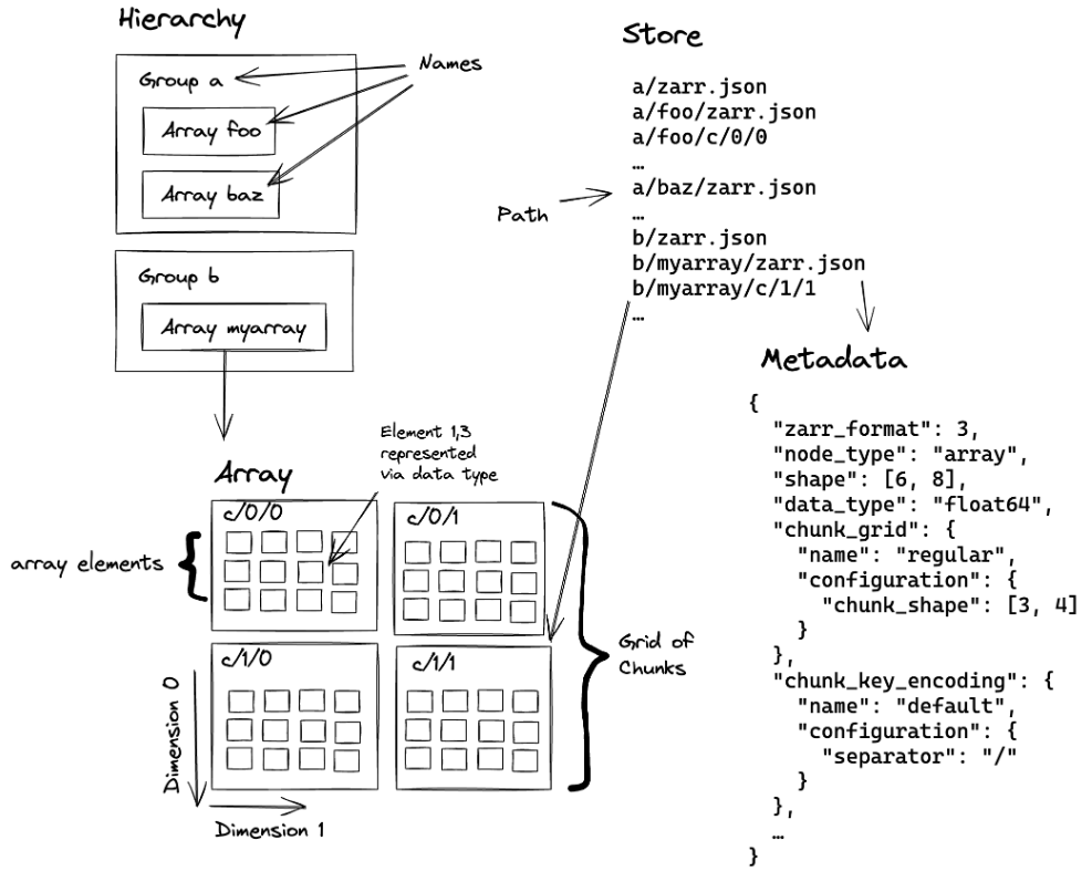
A Zarr dataset is usually organised into three main ideas:

• Arrays: N-dimensional arrays of a single data type, split into chunks.
• Groups: hierarchical containers that can hold arrays and child groups, similar to folders or HDF5 groups.
• Stores: the underlying storage system that holds the data and metadata, such as a local directory, an S3 bucket, or another key-value backend.

A typical climate or ocean dataset might use one group containing arrays such as temperature, salinity, u_wind, and v_wind, each organised by dimensions such as time, lat, lon, and level. Instead of one monolithic file, each array is split into chunks, and each chunk can be stored and read separately.

Source

Zarr v2

Zarr version 2 is the older, widely used storage specification. In Zarr v2, the dataset is organised as a directory-like structure with a few small metadata files plus folders for groups, arrays, and chunks.

At the top level, you usually see:

• .zgroup for group metadata.
• .zattrs for user-defined attributes.
• .zmetadata for consolidated metadata, when enabled.

Inside the group, each array usually appears as its own directory, and that array directory contains:

• .zarray for array metadata.
• .zattrs for array-specific attributes.
• Chunk files, named by their chunk coordinates, such as 0.0.0, 0.0.1, 1.0.0, and so on.

A simple Zarr v2 layout might look like this (please run the following commands in a terminal to see the structure of the Zarr store):

BASH

# Set the base path to your data directory. If you have the data in your current working directory, you can set it to an empty string.
export BASE_DATA_PATH="/gws/ssde/j25b/atlantis_vis/cloud-native-geoscience-course/" # or "" if you have the data in your current working directory

# This command shows the directory structure of a Zarr v2 store for an ocean temperature dataset that we have in the example data folder. You can run this command in a terminal to see the structure of the Zarr store.
tree -L 2 "${BASE_DATA_PATH}data/era5_sst/ocean_temperature_v2.zarr"

OUTPUT

ocean_temperature_v2.zarr/
├── .zattrs
├── .zgroup
├── .zmetadata
├── sst/
│   ├── .zarray
│   ├── .zattrs
│   ├── 0.0.0
│   ├── 0.0.1
│   ├── 0.1.0
│   └── ...
├── valid_time/
│   └── 0
├── longitude/
│   └── 0
└── latitude/
    └── 0

Note: Windows users may need to create an alias to make the tree command work. Please run the following command: echo "alias tree='cmd //c tree //F'" >> ~/.bashrc && source ~/.bashrc.

In this example, sst is one data variable, while valid_time, longitude, and latitude are coordinate arrays. Each array has its own .zarray file describing the array shape, data type, chunk layout, fill value, and other storage settings.

To see the .zgroup, .zattrs, and .zmetadata of this zarr dataset, you can run the following command in a terminal:

BASH

# run the following commands in a terminal

cat "${BASE_DATA_PATH}data/era5_sst/ocean_temperature_v2.zarr/.zgroup"
cat "${BASE_DATA_PATH}data/era5_sst/ocean_temperature_v2.zarr/.zattrs"
cat "${BASE_DATA_PATH}data/era5_sst/ocean_temperature_v2.zarr/.zmetadata"

To see the .zarray metadata for the sst array, you can run:

BASH

cat "${BASE_DATA_PATH}data/era5_sst/ocean_temperature_v2.zarr/sst/.zarray"

This tells us that the sst array is three-dimensional, stored in chunks of size 10 × 100 × 100, and encoded as 32-bit floating-point values. The actual chunk data is stored separately in files such as 0.0.0, 0.0.1, 0.1.0, and so on.

A key feature of Zarr v2 is that the metadata is small, human-readable, and easy to inspect without opening the full dataset. That makes it convenient for browsing dataset structure and understanding how the data are organised before any analysis begins.

Source

Zarr v3

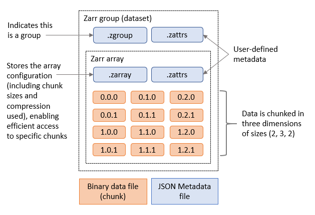
Zarr version 3 is the newer core specification. It keeps the same basic idea of chunked arrays and groups, but it updates the metadata structure and some of the terminology to better support modern scientific and cloud-native use cases.

At a high level, a Zarr v3 store still contains groups, arrays, and chunks, but the metadata is more explicit and consolidated. Instead of several small hidden JSON files spread through a directory tree, Zarr v3 uses zarr.json files to describe groups and arrays. In the metadata itself, the terminology has changed slightly to make it clearer and more flexible. Some important changes from v2 to v3 are:

• dtype becomes data_type.
• chunks becomes chunk_grid.
• dimension_separator becomes chunk_key_encoding.
• order is replaced by the transpose codec.
• filters and compressor are replaced by a more general codecs field.

A simplified Zarr v3 structure might look like this:

BASH

tree -L 2 "${BASE_DATA_PATH}data/era5_sst/ocean_temperature.zarr"

OUTPUT

ocean_temperature.zarr/
├── zarr.json
├── sst/
│   ├── zarr.json
│   └── c
│       ├── 0/0/1
│       ├── 0/1/0
│       └── ...
├── valid_time/
│   ├── zarr.json
│   └── c
│       └── 0
├── longitude/
│   ├── zarr.json
│   └── c
│       └── 0
└── latitude/
│   ├── zarr.json
│   └── c
│       └── 0

In this example, the root zarr.json describes the top-level group, and each array has its own zarr.json file describing its shape, chunk grid, data type, codecs, and other metadata. The chunk data are stored separately under chunk key paths such as c/0/0/0.

Source

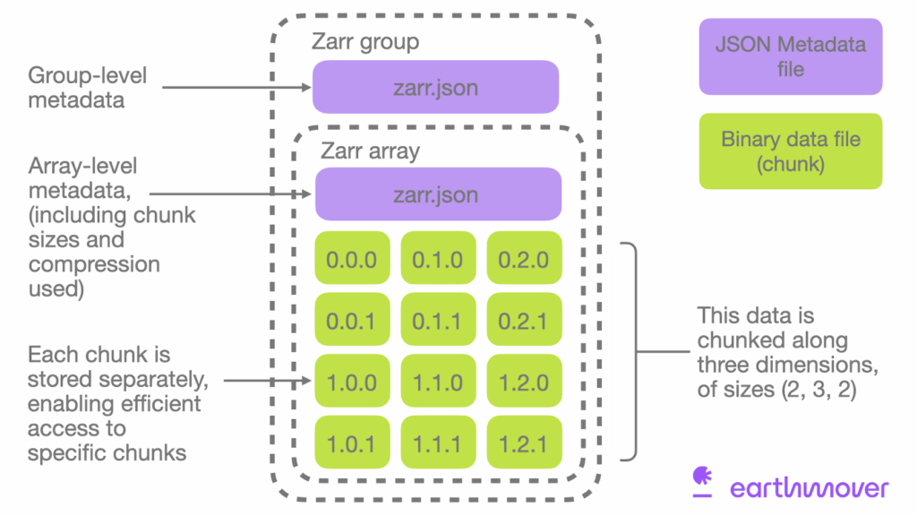
An example of a Zarr v3 metadata file for an array might look like this:

JSON

{
  "zarr_format": 3,
  "data_type": "<f4",
  "shape": [3650, 1800, 3600],
  "chunk_grid": [10, 100, 100],
  "codecs": [
    {
      "id": "zlib",
      "level": 1
    }
  ],
  "fill_value": null,
  "dimension_separator": "/"
}

To see the zarr.json metadata for the root group and for the sst array, you can run:

BASH

cat "${BASE_DATA_PATH}data/era5_sst/ocean_temperature.zarr/zarr.json"
cat "${BASE_DATA_PATH}data/era5_sst/ocean_temperature.zarr/sst/zarr.json"

Zarr v3 also adds more explicit support for features such as sharding, where several chunks can be grouped together inside a larger storage object. This helps reduce the overhead of managing very large numbers of tiny files or keys, especially in cloud object storage. We will talk more about sharding in later lessons.

Chunked storage: how Zarr stores large arrays

---

Chunking is central to Zarr’s design. Instead of storing one very large array as a single block, Zarr splits it into many smaller pieces called chunks. Each chunk is a small N-dimensional block of the array, for example a subset in time × lat × lon, and each chunk can be stored and read separately.

You can think of this like cutting a very large map into tiles. If you only want to look at one region, you do not need to unroll the whole map. You only fetch the tiles you need. Zarr does the same thing for multidimensional data.

For environmental data, chunking is useful because:

• Selective reads: a time series at one point, one region, or one variable can often be read without scanning the whole dataset.
• Parallelism: different chunks can be processed at the same time by different workers.
• Compression: each chunk can be compressed separately, which can reduce storage costs and data transfer.

This is one reason Zarr fits cloud workflows well: object storage and HTTP-based access work naturally when data is organised into many addressable pieces rather than one large monolithic file.

A simple way to think about chunks

Imagine an ocean temperature dataset with dimensions:

• time = 120
• lat = 721
• lon = 1440

If this were stored as one giant array, even small operations could require reading a very large amount of data. With chunking, the dataset can instead be divided into smaller blocks, such as:

• one chunk per group of timesteps,
• one chunk per spatial tile,
• or a combination of both.

When a user asks for “the temperature time series at this point” or “this region for this month”, the software can request only the chunks that overlap that query, rather than the whole array.

How chunking affects data access.

Caution

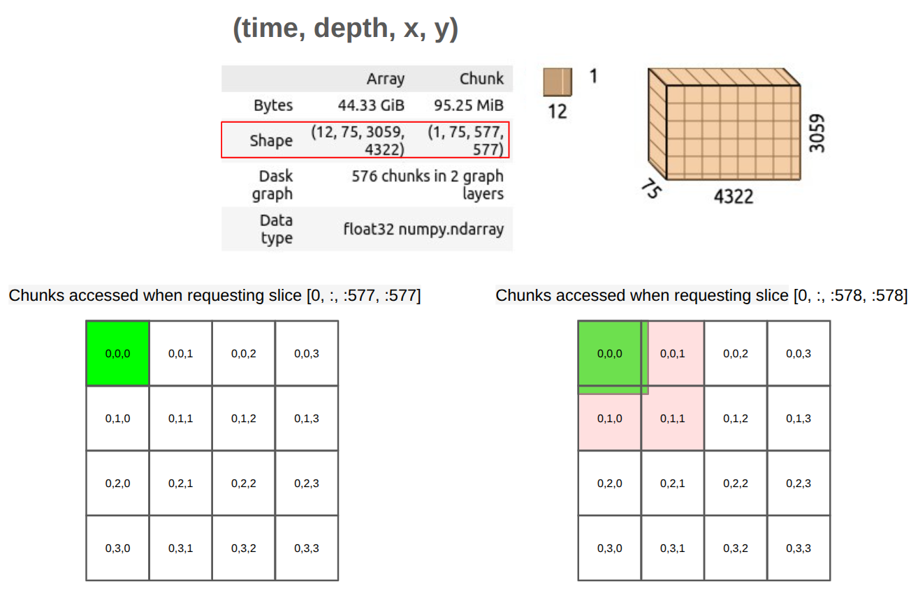
Chunking also has trade-offs

Chunking is powerful, but it is not free. If chunks are too large, each read may bring in much more data than needed. If chunks are too small, the dataset may contain a huge number of tiny objects, and managing all those requests can become inefficient, especially in cloud object storage.

So there is always a balance:

• larger chunks can reduce metadata and request overhead,
• smaller chunks can improve fine-grained access,
• the best chunk shape depends on the kinds of analysis people usually perform.

This trade-off is one reason newer Zarr work has added sharding.

Why Zarr matters for oceanography, climate, and meteorology

---

For these disciplines, Zarr brings several important shifts:

• From files to data cubes: archives can be published as coherent Zarr “stores” representing large data cubes (e.g. global ERA5 climate fields or Sentinel EO products) rather than thousands of individual NetCDF/GRIB files.
• Direct cloud access: scientists can open datasets directly from S3/HTTPS in notebooks or applications, reading only needed chunks instead of downloading entire files.
• Interoperability and tooling: Zarr integrates well with xarray, dask, Icechunk, and visualization tools such as browzarr and zarr-cesium, enabling rich, interactive workflows.
• Community-driven standards: Zarr is being adopted by major providers and projects, and conventions are emerging to ensure interoperability and best practices.

In short, Zarr doesn’t replace scientific semantics like CF or the Common Data Model. It gives us a new storage and access layer that works natively with cloud infrastructure and modern analysis tools.

Inspect a Zarr store with Python

---

To inspect a Zarr store, we can use the zarr library in Python. For example, in the example datasets, we have a Zarr store called data/era5_sst/ocean_temperature_with_groups.zarr. This zarr store represents a subset of the ERA5 reanalysis dataset, with sea surface temperature data organised into pyramid groups and arrays. We will talk later about pyramids and how they are used for multiscale visualisation, but for now we will focus on the Zarr structure itself.

To open this Zarr store, we can run:

PYTHON

import zarr

base_path = "/gws/ssde/j25b/atlantis_vis/cloud-native-geoscience-course/"  # or "" if you have the data in your current working directory

store = zarr.open_group(f"{base_path}data/era5_sst/ocean_temperature_with_groups.zarr", mode="r")
print(store)

To see the arrays and groups inside the store, we can list them:

PYTHON

print(list(store.arrays()))  # List arrays
print(list(store.groups()))  # List groups

Because this Zarr store uses groups, the arrays are not directly in the root group. Instead, they are inside child groups. To see the arrays inside a specific group, we can access that group and list its arrays:

PYTHON

# Show arrays inside group "1"
print(list(store["1"].arrays()))

To see the information about the array sst, we can access it and print its shape, chunk shape, and data type:

PYTHON

# Inspect a specific array
sst = store["1"]["sst"]
print(sst)
print(sst.shape, sst.chunks, sst.dtype)

# Access attributes
print(dict(sst.attrs))

Challenge

Exercise 1 - Inspecting a Zarr store with Python

Using the Zarr store called data/era5_sst/ocean_temperature_with_groups.zarr, please complete the following tasks:

1. Use the Python zarr library to open the store.
2. Inspect the group hierarchy and list available arrays, groups, and their attributes.
3. Identify the dimensions, shape, and data type of the sst array.
4. Explore the metadata files (.zarray, .zgroup, .zattrs or zarr.json) for one array.

Questions:

• How is the store organised (root group, subgroups, arrays)?
• Which variables are stored inside each group?
• What are the shape and data type of the sst array?
• Which attributes are attached to the root group and the sst array?
• Are you loading the dataset into memory, or only inspecting its structure?

Show me the solution

Code to inspect the Zarr store:

PYTHON

import zarr

base_path = "/gws/ssde/j25b/atlantis_vis/cloud-native-geoscience-course/"  # or "" if you have the data in your current working directory

store = zarr.open_group(f"{base_path}data/era5_sst/ocean_temperature_with_groups.zarr", mode="r")

print(store)
print(list(store.groups()))
print(list(store["1"].arrays()))

sst = store["1"]["sst"]
print(sst.shape)
print(sst.dtype)

print(dict(store.attrs))
print(dict(sst.attrs))

Code to list the files and to see the content of the metadata files (as this is a Zarr v3 store, the metadata files are zarr.json):

BASH

# These commands are meant to be run in a terminal, not in Python.
export BASE_DATA_PATH="/gws/ssde/j25b/atlantis_vis/cloud-native-geoscience-course/"  # or "" if you have the data in your current working directory

tree -L 2 "${BASE_DATA_PATH}data/era5_sst/ocean_temperature_with_groups.zarr"
cat "${BASE_DATA_PATH}data/era5_sst/ocean_temperature_with_groups.zarr/zarr.json"
cat "${BASE_DATA_PATH}data/era5_sst/ocean_temperature_with_groups.zarr/1/sst/zarr.json"

The Zarr store is organised as a hierarchical container. In this example, the root group does not contain any arrays directly:

BASH

ocean_temperature_with_groups.zarr
├── 0/
    ├── sst
    ├── valid_time
    ├── latitude
    ├── longitude
    ├── spatial_ref
    ├── number
    └── zarr.json
├── 1/
    └── ...
└── zarr.json

The root Group contains two child groups (0 and 1). The sst variable is stored inside each group 1. The sst array has:

• Shape: (10, 360, 720)
  • 10 time steps
  • 360 latitude points
  • 720 longitude points
• Data type: float32

The array attributes contain metadata inherited from the original GRIB dataset and CF-style information, including long_name -> "Sea surface temperature", for example.

We are not loading the entire dataset into memory. We are only inspecting the structure and metadata. The actual data is read from disk or object storage only when we explicitly request it (e.g., by slicing the array). This lazy loading is a key feature of Zarr and xarray, allowing efficient handling of large datasets.

Challenge

Exercise 2 - Thinking about chunked storage

Using the same Zarr dataset:

1. Inspect the chunk shape of the sst array.
2. Explain what one chunk represents in terms of time and space.
3. Consider how this chunking would affect:
   • reading a time series at one location;
   • computing a spatial mean for each time step.
4. If you were storing a high-resolution global reanalysis, what workloads would you optimise for when choosing chunk shapes?

Show me the solution

To explore the chunk shape of the sst array, you can run:

PYTHON

print(sst.chunks)

A chunk shape such as (10, 100, 100) represents 10 time steps over a 100×100 spatial block. Chunk shapes that are “tall in time” can be efficient for time series at specific locations, while chunk shapes that cover larger spatial regions may be better for spatial aggregates. In practice, chunk shapes are a compromise based on dominant workloads. This exercise prepares you to think critically about chunking decisions, sharding (you will see later what this means), and performance optimisation covered in later lessons (e.g. on cloud-native formats, Zarr V3 features, and tools like Icechunk and Virtualizarr).

Key Points

• “Zarr organises data into groups and arrays stored as addressable chunks, which supports efficient partial reads and writes.”
• “Metadata in Zarr describes array structure, chunking, and attributes, and can be extended through shared conventions for geoscience workflows.”
• “Chunked storage is central to Zarr performance because it lets tools read only the pieces needed for a given query or computation.”
• “Inspecting a Zarr store with Python and xarray helps distinguish cheap metadata exploration from actual data loading.”
• “Understanding data model, metadata, and chunk layout is the foundation for later lessons on rechunking, parallel processing, and cloud-native analysis.”

Content from Python for Zarr

---

Last updated on 2026-08-05 | Edit this page

Overview

Questions

• “What Python packages are commonly used to work with Zarr data?”
• “How can I inspect a Zarr store directly with the zarr library?”
• “How does xarray represent Zarr datasets as labelled N-dimensional data?”
• “When does the data actually get loaded into memory?”
• “What basic xarray operations are useful for oceanography, climate, and meteorology?”

Objectives

• “Import the core Python libraries for working with Zarr data.”
• “Inspect a Zarr store directly with the zarr library.”
• “Open a Zarr dataset with xarray and explore variables, dimensions, and coordinates.”
• “Understand lazy loading and why it matters for large datasets.”
• “Use a few basic xarray operations on environmental Zarr data.”

Python ecosystem for Zarr

---

Zarr has a rich ecosystem of Python tools:

• zarr - the core Python implementation of Zarr’s chunked N‑dimensional arrays and groups.
• xarray - a labelled N‑dimensional array library that can open Zarr datasets and present them as Dataset objects with named dimensions and coordinates.
• fsspec / s3fs / gcsfs / obstore - filesystem adapters to access Zarr stores on local disk, S3, Google Cloud Storage, and other backends.
• Supporting tools - Virtualizarr, Icechunk, and others build on Zarr and xarray for specialised workflows (rechunking, transactional storage, cloud‑ready archives).

In this lesson we focus on the essentials: how to use zarr directly for low-level inspection and how to use xarray for most day‑to‑day analysis with environmental data in Zarr format.

Opening with zarr library

---

As you saw in the previous lesson, Zarr stores are organised into groups and arrays. The zarr library provides low-level access to these stores, allowing you to open groups and arrays, inspect their shapes, chunk shapes, data types, read and write data, and view or edit attributes (metadata).

On the data directory, we have a Zarr store called data/era5_sst/ocean_temperature.zarr. This store contains a single group with one array, representing sea surface temperature data from the ERA5 reanalysis dataset. The array is chunked in time and space, and has metadata attributes such as units and long names.

We can open the Zarr store data/era5_sst/ocean_temperature.zarr using the zarr library:

PYTHON

import zarr

base_path = "/gws/ssde/j25b/atlantis_vis/cloud-native-geoscience-course/"  # or "" if you have the data in your current working directory

root = zarr.open_group(f"{base_path}data/era5_sst/ocean_temperature.zarr", mode="r")
print(root)
print(list(root.arrays()))
print(list(root.groups()))
print("Group attributes:", root.attrs)

You can then inspect one array directly:

PYTHON

temp = root["sst"]
print(temp)
print("Shape:", temp.shape)
print("Chunks:", temp.chunks)
print("Data type:", temp.dtype)
print("Array attributes:", temp.attrs)

A Zarr array tells you how the data are organised on disk or in object storage. Its shape tells you the full size of the array, chunks tells you how it is split up, and attrs can store useful metadata such as units or variable names.

Challenge

Exercise 1 - Explore the store

Using the example Zarr store (data/era5_sst/ocean_temperature.zarr):

1. List all arrays in the root group.
2. Choose one data variable and print its shape, chunks, and dtype.
3. Inspect the array attributes and identify at least three useful metadata fields.

Questions:

• What dimensions do you think the shape represents?
• How does chunks divide the data?
• Which attributes look useful for analysis?

Show me the solution

Each array has a fixed shape and chunk layout, and that metadata provides context such as units, long names, and standard names:

PYTHON

import zarr

root = zarr.open_group(f"{base_path}data/era5_sst/ocean_temperature.zarr", mode="r")
print(list(root.arrays()))
sst = root["sst"]
print(sst)
print("Shape:", sst.shape)
print("Chunks:", sst.chunks)
print("Data type:", sst.dtype)
print("Array attributes:", sst.attrs)

Callout

Lazy loading and memory

Opening a Zarr store usually reads metadata first, not the full data values. This is often called lazy loading: the dataset structure is available immediately, but the chunk data are only read when you ask for values.

With zarr, properties such as shape, chunks, dtype, and .attrs come from metadata. The actual data are read when you index or slice the array.

PYTHON

first_slice = temp[0, :, :]

At that point, Zarr reads only the chunks needed for that selection. It does not need to load the full array unless you request the full array.

The same idea applies with xarray: opening the dataset is cheap, and data are loaded only when you select, compute, plot, or ask for values.

Opening with xarray

---

While zarr is ideal for low-level inspection and manipulation, xarray is usually the main tool for analysing multidimensional environmental data. It provides:

• Datasets - collections of data variables (arrays) with shared dimensions and coordinates.
• Labelled dimensions - names like time, lat, lon, depth instead of numeric indices.
• Coordinates - explicit arrays for latitude, longitude, time, etc.
• High-level operations - selection (.sel), reduction (.mean, .sum), resampling, plotting, etc.

Xarray

xarray can open NetCDF, GRIB (via backends), and Zarr data. Because of this, it makes Zarr datasets accessible in a familiar, analysis-ready format. And it also makes it really easy to update workflows to use cloud-native Zarr stores without changing the analysis code.

For Zarr it uses xr.open_zarr, which understands the Zarr metadata and conventions. Basic usage:

PYTHON

import xarray as xr

ds = xr.open_zarr(f"{base_path}data/era5_sst/ocean_temperature.zarr")
print(ds)           # Overview of variables and coordinates
print(ds.dims)      # Dimensions
print(ds.data_vars) # Data variables
print(ds.coords)    # Coordinate variables

Important points:

• ds is an xarray Dataset.
• ds.data_vars lists data variables (e.g. sst, salinity).
• ds.coords typically includes time, lat, lon, and any other coordinate variables.
• Metadata from Zarr arrays and attributes is mapped into xarray’s structure so that CF conventions and other patterns can be used.

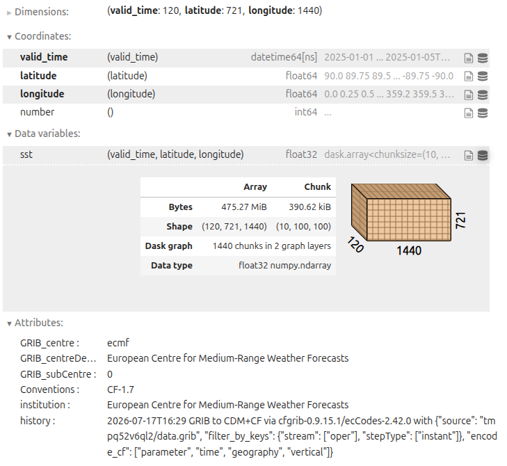
The result is an xarray Dataset. Each variable is an xarray DataArray, and the metadata from the Zarr store is carried into the xarray structure.

PYTHON

sst = ds["sst"]
print(sst)
print("SST dims:", sst.dims)
print("SST attrs:", sst.attrs)

Zarr in Xarray

Challenge

Exercise 2 - Open with xarray

Using the same dataset:

1. Open it with xr.open_zarr.
2. Print ds.dims, ds.data_vars, and ds.coords.
3. Inspect one variable and print its dimensions and attributes.
4. Note whether the dataset opens quickly even if it is large.

Questions:

• Which variables are data variables versus coordinates?
• Which dimensions are present?
• What does xarray tell you about the dataset without loading all the values?

Show me the solution

PYTHON

import xarray as xr
ds = xr.open_zarr(f"{base_path}data/era5_sst/ocean_temperature.zarr")
print(ds.dims)
print(ds.data_vars)
print(ds.coords)

Xarray organises the dataset into named dimensions and separates data variables from coordinate variables, which makes the structure easier to understand. Opening the dataset is fast because xarray reads metadata first and loads data only when needed.

Callout

NetCDF vs Zarr with xarray

If we open the same dataset in NetCDF format, we can use xr.open_dataset:

PYTHON

ds_netcdf = xr.open_dataset(f"{base_path}data/era5_sst/ocean_temperature.nc")
print(ds_netcdf)

You will see that the structure is very similar to the Zarr version. The main difference is that NetCDF is a single file, while Zarr is a directory of chunked arrays. But xarray provides a consistent interface for both formats, so analysis code can be reused.

Basic xarray operations

In oceanography, climate, and meteorology, we often want to select data by coordinates, compute means over dimensions, and plot results. Xarray provides a simple interface for these operations:

• Select data with .sel() using coordinate values.
• Use .isel() when you want numeric positions.
• Compute a mean over one or more dimensions (e.g. .mean(dim=("latitude", "longitude"))).
• Plot a slice quickly with .plot().

PYTHON

time_slice = ds["sst"].sel(valid_time=slice("2025-01-01T00:00:00", "2025-01-02T00:00:00"))
global_mean = ds["sst"].mean(dim=("latitude", "longitude"))
point_ts = ds["sst"].sel(latitude=0.0, longitude=0.0, method="nearest")
isel_slice = ds["sst"].isel(valid_time=0, latitude=200, longitude=200)

In the operations above, the data is not loaded into memory until you request values or plot the results. For example, the following code will trigger data loading and plotting:

PYTHON

# map plot
time_slice.sel(valid_time="2025-01-01T00:00:00").plot()

PYTHON

# time series plot
point_ts.plot()

PYTHON

# just to see a point value
print(isel_slice.values)

These operations are especially useful for environmental data, because they keep the code readable and let you work with named coordinates rather than raw array positions.

What comes into memory?

A useful rule of thumb is:

• Opening a Zarr store loads metadata.
• Inspecting shape, chunks, dims, and attributes mostly uses metadata.
• Selecting, computing, plotting, or calling .values reads data chunks into memory.

For example, this mainly inspects metadata:

PYTHON

print(ds["sst"])
print(ds["sst"].dims)
print(ds["sst"].attrs)

But this requests actual data values:

PYTHON

ds["sst"].isel(valid_time=0).values

This distinction is one of the main reasons Zarr works well for large environmental datasets: you can explore the dataset structure first, and only load the parts you need for analysis.

Challenge

Exercise 3 - First analysis on a Zarr dataset

Using the data/era5_sst/ocean_temperature.zarr dataset and xarray:

1. Inspect the available variables and pick the sea surface temperature.
2. Compute a spatial mean over latitude and longitude and inspect the resulting time series.
3. Select a small spatial region (e.g. a box around a particular ocean basin) and compute a mean for that region. Remember that you have to use max_lat before min_lat in slice() because latitude decreases from north to south. And remember that longitude is usually 0-360 in ERA5.

Questions:

• How does xarray’s interface make these operations readable compared to direct array indexing?
• What would change if the dataset were too large to fit in memory (you’ll explore this in later lessons with Dask and cloud‑native formats)?
• How comfortable do you feel with xarray’s basic usage now?

Show me the solution

PYTHON

import xarray as xr

ds = xr.open_zarr(f"{base_path}data/era5_sst/ocean_temperature.zarr")

sst = ds["sst"]

# Global mean time series
global_ts = sst.mean(dim=("latitude", "longitude"))
print(global_ts)

# Regional mean (example box)
regional_ts = sst.sel(latitude=slice(0, -30), longitude=slice(300, 360)).mean(dim=("latitude", "longitude"))
print(regional_ts)

# Additional plotting if desired
regional_ts.plot()

Xarray’s labelled dimensions and high‑level methods (.mean, .sel, .plot) make common operations much more expressive and less error‑prone than raw array indexing. Opening Zarr datasets with xarray offers a consistent interface across storage formats, laying the groundwork for later lessons on performance, chunking, and cloud‑native workflows.

Challenge

Exercise 3 - Read only a small part

Use xarray to open the Zarr dataset, then select only a small part of it. Select temperature data for the first hour of 2025, for a small region in the Brazilian Southest Coast (min lat: -30, max lat: -20, min lon: -50, max lon: -40). Compute the mean of that subset.

Questions:

• Did you need to load the full dataset?
• What parts were actually read into memory?
• Why is this useful for large datasets?
• What would be the comparison if you had to load a NetCDF file instead?

Show me the solution

PYTHON

import xarray as xr

ds = xr.open_zarr(f"{base_path}data/era5_sst/ocean_temperature.zarr")
sst = ds["sst"]

subset = sst.sel(valid_time="2025-01-01T00:00:00", latitude=slice(-20, -30), longitude=slice(310, 320))  # Note: longitude is 0-360 in ERA5, so -50 to -40 becomes 310 to 320
print(subset)
print(subset.mean().values)

We can open a huge dataset and still process only a small portion of it. This is one of the main advantages of Zarr and xarray for large environmental data.

Key Points

• “The zarr Python package provides low-level access to Zarr stores, including groups, arrays, and attributes.”
• “xarray is the main high-level tool for working with environmental Zarr datasets as labelled N-dimensional data.”
• “Opening Zarr with xarray (xr.open_zarr) gives you variables, dimensions, and coordinates in a familiar Dataset structure.”
• “Data values are loaded only when they are selected or used in a computation.”
• “Basic xarray operations such as selection, reduction, and plotting work the same on Zarr data as on NetCDF data.”

Content from Choosing Chunks at Scale

---

Last updated on 2026-08-05 | Edit this page

Overview

Questions

• “What is a chunk, and why does its shape matter for performance?”
• “How should I choose chunk sizes for different types of analysis?”
• “What are the trade-offs between large and small chunks?”
• “How can I rechunk a Zarr dataset and save it for future use?”
• “What is sharding, and how does it help reduce overhead during storage and access of many small chunks?”

Objectives

• “Understand what chunks are and how they affect performance for large datasets.”
• “Relate common analysis workflows (time series, spatial averages, ensembles) to chunk layouts.”
• “Use Python (zarr and xarray) to inspect chunk shapes in a Zarr store.”
• “Rechunk a Zarr dataset, save it, and observe how analysis performance changes.”
• “Understand the concept of sharding and how it can reduce overhead in cloud object storage.”

What are chunks?

---

In Zarr (and in many array-based systems), a chunk is a small N-dimensional block of an array that is stored and accessed as a unit. Instead of storing one giant array in a single file or object, we:

• Divide the array into chunks (e.g. (time, lat, lon) = (10, 100, 100) per chunk).
• Store each chunk separately (e.g. as a separate object in a directory or bucket).
• Read and write data chunk-by-chunk when we need it.

Chunks influence:

• I/O patterns: which parts of the dataset are read from storage.
• Parallelism: how work can be distributed across many processes or threads.
• Compression effectiveness: how well data compresses within each chunk.
• Metadata overhead: number of chunks and associated bookkeeping.

Choosing good chunk shapes is critical when you move from “toy” datasets to large-scale reanalysis, ensemble, or high-resolution model data.

Thinking in dimensions and workloads

To choose chunk shapes, start from your dimensions and typical workloads.

Common dimensions in ocean, climate, and meteorology:

• time
• lat, lon (or x, y)
• level (or depth) (pressure or model levels, depth in the ocean)
• member (ensemble member)

Common workloads:

• Time series at a point: e.g. temperature at one location over many years.
• Spatial averages per time step: e.g. global mean temperature as a function of time.
• Regional subsets: e.g. data over a specific basin or region.
• Vertical profiles: e.g. temperature vs. depth at a given location and time.
• Ensemble statistics: e.g. mean and spread across member.

Each workload benefits from certain chunk layouts:

• Time series: chunks that include many time steps for a small spatial region.
• Spatial averages per time step: chunks that include complete spatial slices (or large spatial blocks) for a small number of time steps.
• Ensemble statistics: chunks that include multiple ensemble members together, if members are frequently used together.
• Cloud/web visualisation: use smaller, spatially aligned chunks, often around 256×256 or 512×512 pixels (~100-1000 KB size), so that map tiles can be read efficiently and only the needed region is transferred.
• Large HPC analysis: use larger chunks that reduce scheduler overhead and work well with parallel processing, but still fit in memory comfortably (e.g. 10-100 MB size).

There is no single “best” chunking: it depends on which workloads are most important for your users.

Source

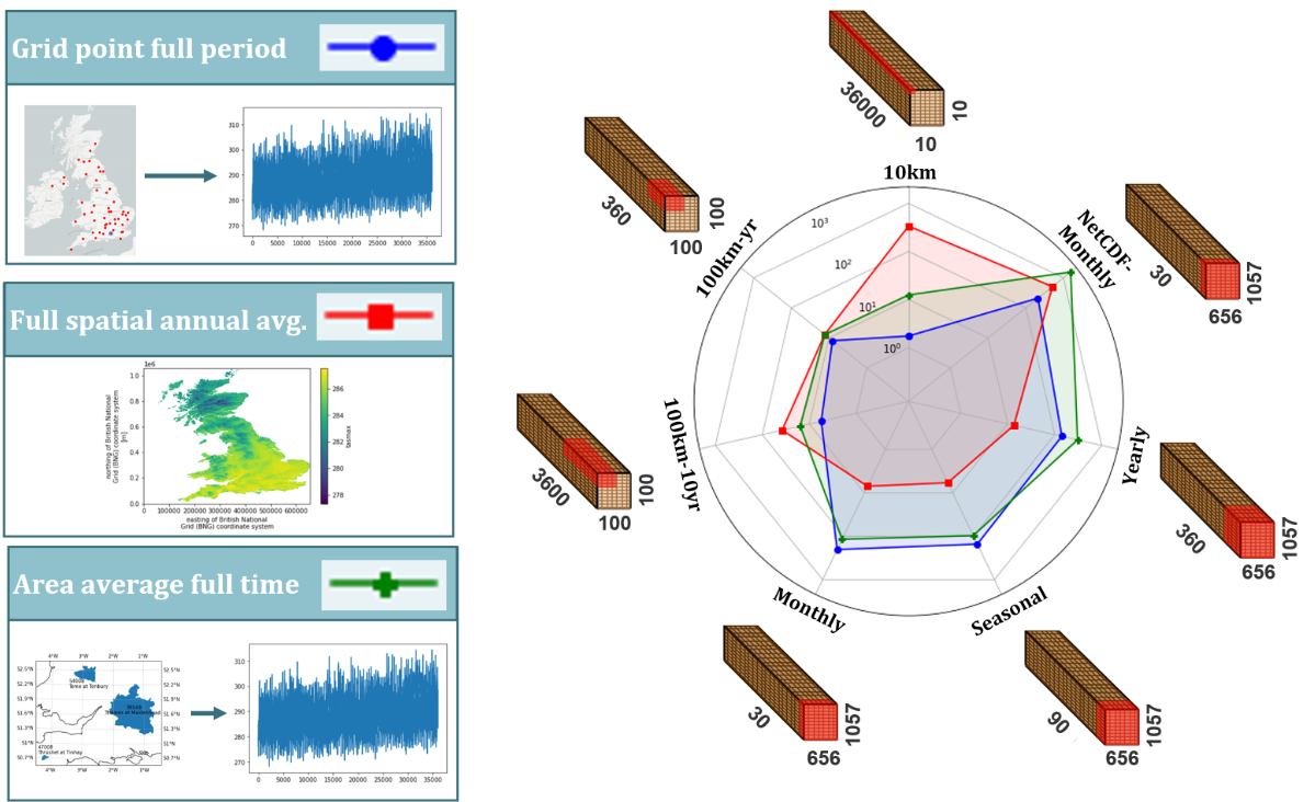
Inspecting chunk shapes in a Zarr store

---

Let’s take a look on one of our example Zarr datasets to see how chunks are laid out. Now we are using a subset of the GLORYS12V1 Ocean Reanalysis dataset. The GLORYS12V1 product is the CMEMS global ocean eddy-resolving (1/12° horizontal resolution, 50 vertical levels) reanalysis covering the altimetry period from 1993 onward.

The subset is stored in a single Zarr group, and it is available in the data/glorys/ directory.

PYTHON

import xarray as xr

base_path = "/gws/ssde/j25b/atlantis_vis/cloud-native-geoscience-course/" # or "" if you have the data in your current working directory

ds = xr.open_zarr(f"{base_path}data/glorys/glorys_202605.zarr")
print(ds)

Now, let’s inspect the zos variable (Sea surface height) and see its dimensions, shape, and chunking:

PYTHON

zos = ds["zos"]
print("Dimensions:", zos.dims)
print("Shape:", zos.shape)
print("Chunks:", zos.data.chunks)

Seeing shape and dims helps you reason about how the current chunking might align with your workloads.

Challenge

Exercise 1 - Relate current chunking to workloads

Using the GLORYS12V1 Ocean Reanalysis example Zarr dataset (data/glorys/glorys_202605.zarr), answer the following:

1. Inspect the so (Salinity) array’s shape and chunks using xarray.

2. Map the dimensions to names (e.g. interpret (time, lat, lon, depth) from context or attributes and following the CF conventions).

3. For each of these workloads, decide whether the current chunking seems “friendly” or “unfriendly”:

   • Time series at a point.
   • Spatial mean per time step.
   • Regional subset (e.g. a North Atlantic box).
   • Vertical profile at a point.

Show me the solution

PYTHON

# shape
print(ds["so"].shape)

# chunks
print(ds["so"].data.chunks)

# dimensions
print(ds["so"].dims)

Following the coordinate names and CF conventions (standard_name="sea_water_salinity"), the dimensions represent:

so(time, depth, latitude, longitude)

where:

• time = time steps
• depth = vertical ocean levels
• latitude = north-south position
• longitude = east-west position

The current chunking stores one time step and one depth level with the complete global horizontal grid.

It is friendly for workloads that need the full spatial field at a given time (e.g. computing a global mean), but unfriendly for workloads that need many time steps or many depth levels at a single point, because it requires reading many large chunks to get a small amount of data.

It is not friendly for regional subsets either, because the latitude and longitude dimensions are not chunked, so even a small region requires reading the whole global spatial chunk.

It is also not friendly for time series at a point, because the data is split into separate time chunks, and each chunk contains the full spatial field. To get a time series at a single point, you would need to read many large chunks, which is inefficient.

It is not friendly for vertical profiles at a point either, because we have each depth level in separate chunks, and each chunk contains the full spatial field. To get a vertical profile at a single point, you would need to read many large chunks, which is inefficient.

This example shows that chunking is a trade-off: the current layout is good for global spatial operations but inefficient for point-based time series, regional analysis, or vertical profiles.

Callout

Trade-offs: small vs large chunks

Some general guidelines:

• Chunk size in bytes: often a target of a few MB per chunk (e.g. 1-100 MB), depending on storage and compute environment.
  • Too small: many tiny reads and lots of metadata overhead.
  • Too large: slow reads and poor parallelism, especially over networks.
• Chunk shape in dimensions:
  • Align chunks with common access patterns (e.g. contiguous in time for time series, or contiguous in space for spatial stats).
  • Avoid chunking along rarely used dimensions (e.g. member or level) unless you often process across them.

Rechunking

---

Rechunking means changing the way a dataset is divided into chunks. This matters because the best chunk layout depends on how the data will be used: for example, one layout may be better for reading time series, while another may be better for reading maps or writing cloud-optimized storage.

With xarray, rechunking is simple, but it can be expensive for large datasets. The basic steps are:

Step 1: Open the dataset

Start by opening the original Zarr dataset. For the examples below, we will use the ERA5 reanalysis dataset, because it is smaller and easier to work with than the GLORYS dataset (you can try larger datasets later if you want).

PYTHON

import xarray as xr

ds = xr.open_zarr(f"{base_path}data/era5_sst/ocean_temperature.zarr")
print(ds)

You can see that this dataset has dimensions (valid_time, latitude, longitude) and is chunked in a certain way. You can inspect the shape and the chunking of the sst (sea surface temperature) variable:

PYTHON

print(ds["sst"].shape)
print(ds["sst"].chunks)

OUTPUT

(120, 721, 1440)
((10, 10, 10, 10, 10, 10, 10, 10, 10, 10, 10, 10), (100, 100, 100, 100, 100, 100, 100, 21), (100, 100, 100, 100, 100, 100, 100, 100, 100, 100, 100, 100, 100, 100, 40))

Step 2: Choose a new chunk layout

Decide how you want the dataset to be chunked. For example, you might want to have chunks that are larger in space but represents only one time step:

PYTHON

ds_chunked = ds.chunk({"valid_time": 20, "latitude": 180, "longitude": 180})

Step 3: Check the new chunking

Inspect the rechunked dataset to confirm that the chunk layout looks right.

PYTHON

print(ds_chunked)
print(ds_chunked["sst"].chunks)

Step 4: Write the rechunked data to a new Zarr store

Save the dataset with the new chunk layout. However, because this dataset also has an encoding for the sst variable, you also need to update the encoding to reflect the new chunking.

Note that we are going to save the data in your local data directory (not in the base_path):

PYTHON

ds_chunked.to_zarr(
  "data/era5_sst/ocean_temperature_rechunked.zarr",
  mode="w",
  encoding={"sst": {"chunks": (20, 180, 180)}},
)

This approach is convenient, but it is not always the most efficient for very large datasets. If the original and target chunk layouts are very different, rechunking can require substantial temporary storage and memory. And we will also create a new Zarr store, which may be expensive in terms of storage.

Callout

Rechunking with Rechunker or Cubed

Rechunker is a library designed specifically for rechunking large array datasets efficiently. It is useful when you want to move from one chunk layout to another without loading the whole dataset into memory at once. However, rechunker does not work with zarr v3 stores.

Cubed is a newer library that provides an array API for rechunking and other operations, designed to work with serverless backends or locally without needing a live Dask scheduler.

You can also integrate Cubed with xarray to rechunk datasets in a more memory-efficient way.

PYTHON

ds_chunked = ds.chunk({"valid_time": 1, "latitude": 721, "longitude": 1440}, chunked_array_type="cubed")

Rechunk can be expensive

---

In some cases, rechunking can take a long time, especially if the original and target chunk layouts are very different. For example, a study on Zarr data¹ in cloud-based object stores calculated the time to rechunk a 9–10 GB dataset with different chunking strategies:

Chunking strategy	Rechunk time
Large chunks	~6.66 min
Recommended compromise (best overall access pattern)	~22.44 min
Very small chunks	~46 h

Challenge

Exercise 2 - Designing a new chunk scheme

Using the same dataset (ocean_temperature.zarr), think through the following:

1. Identify your priority workload for this dataset (e.g. time series analysis, spatial means, ensemble statistics).
2. Propose a chunk scheme (e.g. {"valid_time": 20, "latitude": 180, "longitude": 180}) that you expect to work well for that workload.
3. Consider the likely chunk size in bytes (rough estimation is fine) and whether it seems reasonable (not too small, not too large). To calculate the approximate chunk size, you can use:

PYTHON

import numpy as np

chunk_shape = (20, 180, 180)  # example chunk shape
chunk_size_bytes = np.prod(chunk_shape) * ds["sst"].dtype.itemsize
print(f"Approximate chunk size: {chunk_size_bytes / 1e6:.2f} MB")

You do not need to run the code yet, focus on design:

• Write down your proposed chunk sizes per dimension.
• Explain how they help your chosen workload.
• Note any trade-offs you are making for other workloads.

Show me the solution

You should choose chunk sizes that reflect their dominant workloads and keep chunk sizes in a plausible range. For example:

• Time series analysis: you might choose relatively large time chunks and moderate spatial blocks. E.g. {"valid_time": 120, "latitude": 10, "longitude": 10} would give you all time steps per chunk and a 10×10 spatial block.
• Spatial analysis: you might choose chunks that cover entire latitude or longitude bands. E.g. {"valid_time": 1, "latitude": 721, "longitude": 1440} would give you one time step per chunk and the full spatial grid.

Recognising that one dataset may need different chunking schemes for different scenarios is a key insight.

Challenge

Exercise 3 - Rechunk and compare

Try the following on your example dataset:

1. Implement a rechunking scheme you designed in Exercise 2, saving to a new Zarr store.
2. Measure the time to compute:
   • A global mean time series (mean(dim=("latitude", "longitude"))).
   • A regional mean time series (e.g. a subset in latitude/longitude).
3. Compare the timings between the original and rechunked stores. To calculate the time taken for each operation, you can use the %%time magic in a Jupyter notebook, or the time module in a script:

PYTHON

import time

t0 = time.time()
# your operation here with the original store
t1 = time.time()
print("Original store time:", t1 - t0, "seconds")

t0 = time.time()
# your operation here with the rechunked store
t1 = time.time()
print("Rechunked store time:", t1 - t0, "seconds")

4. Discuss how chunk layout might matter for larger datasets or cloud environments.

Show me the solution

PYTHON

import time
import xarray as xr

# Open the original and rechunked datasets
ds_original = xr.open_zarr(f"{base_path}data/era5_sst/ocean_temperature.zarr")
ds_rechunked = xr.open_zarr("data/era5_sst/ocean_temperature_rechunked.zarr")

# Measure time for global mean time series
t0 = time.time()
global_mean_original = ds_original["sst"].mean(dim=("latitude", "longitude")).compute()
t1 = time.time()
print("Original store global mean time:", t1 - t0, "seconds")

t0 = time.time()
global_mean_rechunked = ds_rechunked["sst"].mean(dim=("latitude", "longitude")).compute()
t1 = time.time()
print("Rechunked store global mean time:", t1 - t0, "seconds")

You may observe modest timing differences. This is because the dataset is small enough that the overhead of reading chunks is not significant. However, for larger datasets or when working in cloud environments, the chunk layout can have a much more pronounced effect on performance and cost. The key takeaway is that chunking is not just a storage detail: it can have a real impact on compute cost, especially when running at scale on large climate or ocean datasets in the cloud.

Sharding: grouping chunks together

---

Sharding is a way to keep the logical benefits of small chunks while reducing the physical cost of storing too many tiny objects.

A simple way to explain it is:

• Chunks control the unit of computation and data access.
• Shards control how many chunks are packed into each stored object.

You can think of chunks as individual pages, and a shard as a binder holding many pages. We still read the page we need, but we do not have to store every page as its own separate file.

This is especially useful in cloud object storage, where millions of very small objects can be inefficient to manage. With sharding, Zarr can keep a fine-grained internal chunk structure for analysis, while storing multiple chunks together in fewer, larger objects.

This means you can keep chunks small for efficient analysis, while using sharding to avoid creating an excessive number of files or objects.

A sharded Zarr showing how chunk data is grouped into shard files. Source: https://element84.com/software-engineering/is-zarr-the-new-cog/

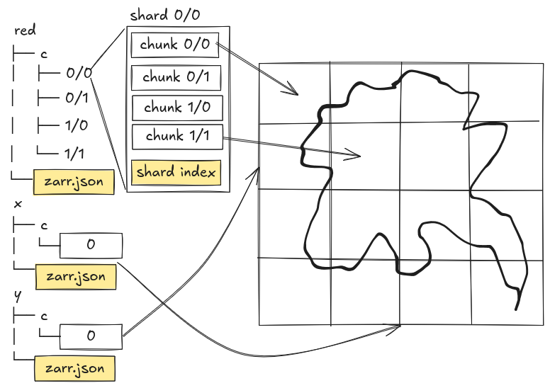
Benefits

Sharding can be useful when:

• You want small chunks for fast, selective reads.
• You want to reduce object counts in cloud storage.
• You want to reduce filesystem overhead from very large numbers of files.
• You want to keep the benefits of chunk-based analysis without paying the full cost of storing each chunk separately.

Trade-offs

Sharding is not always the best choice. If your workload frequently reads only a tiny part of one shard, you may transfer more data than necessary. Sharding also makes partial writes more complicated, because updating one chunk may require rewriting part of a shard.

For that reason, shard layout should reflect the way the data will actually be used. For example, if users usually read neighbouring map tiles together, you might group spatial chunks into the same shard. If they usually read time series, you might group chunks along time instead.

Zarr v3 sharding example

Zarr Python v3 supports sharded arrays directly when you create the array. In the example below, the array has small chunks for analysis, but those chunks are grouped into larger shards for storage.

Let’s create a sharded Zarr array with 10×10 chunks, but store them in 100×100 shards:

PYTHON

import numpy as np
import xarray as xr

data = np.random.randint(0, 100, size=(1000, 1000)).astype("int32")
ds = xr.Dataset({"temperature": (("y", "x"), data)})

ds.to_zarr(
    "data/example_sharded.zarr",
    mode="w",
    zarr_format=3,
    encoding={"temperature": {"chunks": (10, 10), "shards": (100, 100)}},
)

In this example:

• chunks=(10, 10) means the data are split into small 10×10 chunks for fine-grained access.
• shards=(100, 100) means many of those chunks are packed into a larger 100×100 shard for storage.

You can open the array again and inspect it in the same way:

PYTHON

ds = xr.open_zarr("data/example_sharded.zarr")
print(ds)
print(ds["temperature"].chunks)
print(ds["temperature"].encoding)

You can see that the chunking is still (10, 10), but the underlying storage is grouped into larger shards. You can also inspect the Zarr metadata directly:

BASH

# Run this command in your terminal to see the Zarr metadata for the sharded array
cat data/example_sharded.zarr/temperature/zarr.json

OUTPUT

{
  "shape": [
    1000,
    1000
  ],
  "chunk_grid": {
    "name": "regular",
    "configuration": {
      "chunk_shape": [
        100,
        100
      ]
    }
  },
  "chunk_key_encoding": {...},
  "codecs": [
    {
      "name": "sharding_indexed",
      "configuration": {
        "chunk_shape": [
          10,
          10
        ],
        "codecs": [...]
      }
    }
  ],
  ...
  "zarr_format": 3,
}

Two fields matter:

• “chunk_grid.configuration.chunk_shape”: this is actually the shard shape ([100, 100] in our case).
• “codecs”: look for the entry with "name": "sharding_indexed". Its configuration.chunk_shape ([10, 10]) is the real sub-chunk size inside each shard, along with the compressor used.

Using xarray with sharded Zarr

Xarray can open a sharded Zarr store the same way it opens other Zarr datasets, so the sharding is mostly a storage detail from the analyst’s point of view.

PYTHON

import xarray as xr

ds = xr.open_zarr("data/example_sharded.zarr")
print(ds)

temp = ds["temperature"]
print(temp.dims)
print(temp.shape)
print(temp.chunks)

This is useful because xarray still lets you work with labelled dimensions and high-level operations, while Zarr v3 handles the storage layout underneath.

Challenge

Exercise 4 - Shard the dataset

1. In the rechunked dataset you created in Exercise 3, implement a sharding scheme that groups multiple chunks into larger shards. For example, if your chunks are (20, 180, 180), you might choose to shard them into (100, 360, 360). Because you are changing the chunks (by setting the shards parameter in the encoding), you need to use align_chunks=True when saving the dataset to Zarr:

PYTHON

ds_rechunked.to_zarr(..., align_chunks=True)

2. Inspect the Zarr metadata to confirm that the shards are being used, and that the chunking is still as you expect.
3. Compare the number of files/objects in the original, rechunked, and sharded datasets. You can use the example below to perform this calculation:

PYTHON

zarr_store_path = Path(f"{base_path}data/era5_sst/ocean_temperature.zarr/sst/c") # use the "c" directory as it contains the actual chunk data
print("Total Files:", sum(1 for p in zarr_store_path.rglob("*") if p.is_file()))

Show me the solution

PYTHON

import os
import xarray as xr

# Open the rechunked dataset
ds_rechunked = xr.open_zarr("data/era5_sst/ocean_temperature_rechunked.zarr")

ds_rechunked = ds_rechunked.chunk({"valid_time": 20, "latitude": 180, "longitude": 180})
# Save the dataset with sharding
ds_rechunked.to_zarr("data/era5_sst/ocean_temperature_sharded.zarr", mode="w", zarr_format=3,
                     encoding={"sst": {"chunks": (20, 180, 180), "shards": (100, 360, 360)}}, align_chunks=True)

# Inspect the Zarr metadata
ds_sharded = xr.open_zarr("data/era5_sst/ocean_temperature_sharded.zarr")
print(ds_sharded)
print(ds_sharded["sst"].chunks)

To calculate the number of files/objects in each dataset, you can use the following code:

PYTHON

original = Path(f"{base_path}data/era5_sst/ocean_temperature.zarr/sst/c")
rechunked = Path(f"data/era5_sst/ocean_temperature_rechunked.zarr/sst/c")
sharded = Path(f"data/era5_sst/ocean_temperature_sharded.zarr/sst/c")
print("Original:", sum(1 for p in original.rglob("*") if p.is_file()))
print("Rechunked:", sum(1 for p in rechunked.rglob("*") if p.is_file()))
print("Sharded:", sum(1 for p in sharded.rglob("*") if p.is_file()))

Using this approach, you should see that the sharded dataset has fewer files/objects than the original and rechunked datasets, while still maintaining the benefits of chunked access for analysis.

Caution

Remember:Chunking and sharding are not the same

Chunking answers the question: what is the unit of computation and access?

Sharding answers the question: how are those chunks physically packed into storage objects?

A dataset may use small chunks for flexible analysis, but store those chunks inside larger shards to make cloud storage more efficient.

Key Points

• “Chunks are N-dimensional blocks that control how data is stored and accessed in Zarr.”
• “Chunk shapes should be chosen based on dominant workloads (time series, spatial averages, ensembles) and practical constraints like chunk size in bytes.”
• “Rechunking can reorganise a dataset to better match performance needs, at the cost of an initial rewrite step.”
• “Tools like zarr and xarray make it possible to inspect chunk layouts, design new schemes, and save rechunked Zarr stores for analysis at scale.”
• “Sharding is a technique that groups multiple chunks into larger storage objects, reducing overhead while keeping the benefits of chunked access.”

---

1. Nguyean, T., et al. (2023). Impact of Chunk Size on Read Performance of Zarr Data in Cloud-based Object Stores. https://essopenarchive.org/doi/full/10.1002/essoar.10511054.2↩︎

Content from Parallel Processing with Zarr

---

Last updated on 2026-08-05 | Edit this page

Overview

Questions

• “Why do we need parallel processing for large Zarr datasets?”
• “How does Dask parallelise xarray and Zarr computations?”
• “How do chunking and lazy loading support parallel work?”
• “What other parallelism tools do Python users sometimes combine with Zarr?”

Objectives

• “Explain why parallel processing matters for large Zarr datasets.”
• “Use Dask with xarray and Zarr to parallelise common array computations.”
• “Understand how chunking, lazy loading, and task graphs work together.”
• “Recognise a few other Python parallelism patterns that are sometimes used with Zarr workflows.”

Why parallel processing?

---

Large environmental datasets can be too slow or too large to process on a single core or in a single process. This becomes especially important with Zarr because the format is designed to be read and written chunk-by-chunk, which makes it a natural fit for parallel work.

Processing such data on a single core or in a single process can be:

• Slow: long runtimes for even simple operations.
• Memory-limited: datasets or intermediate results may not fit into RAM.
• I/O-bound: reading and writing data dominates computation time, especially from disks or across networks.

Parallel processing helps when your workflow needs to:

• read many chunks from a Zarr store,
• compute statistics over large spatial or temporal regions,
• or run the same operation over many independent files, variables, or ensemble members.

In practice, parallelism works best when both the compute layer and the data layout are aligned. Chunked storage such as Zarr lets multiple workers read different chunks independently, while Dask can schedule the work across those chunks.

Source

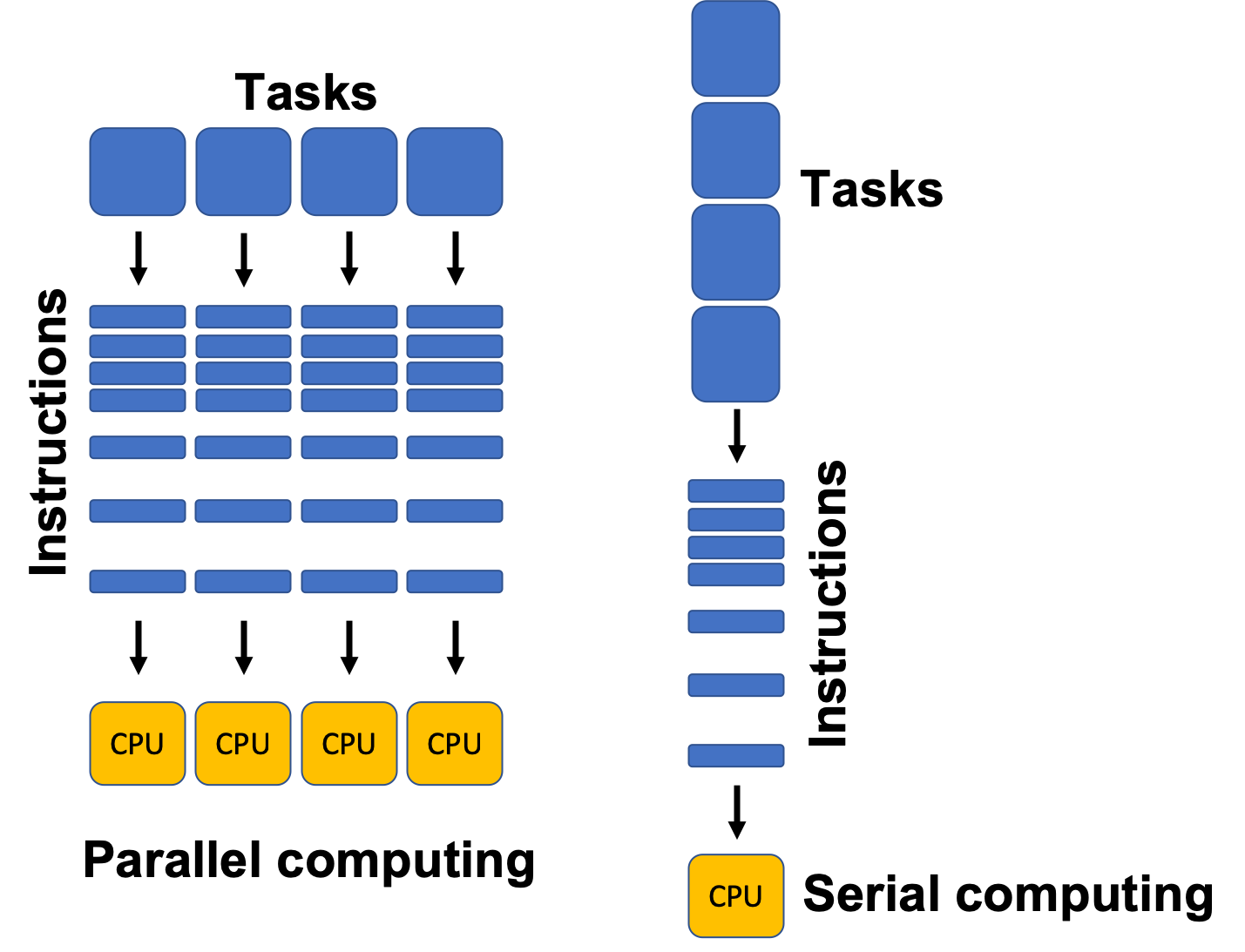
Dask: distributed processing for Python

---

Dask is a distributed processing library for Python. It enables parallel processing of Python code across multiple cores on the same computer or across multiple computers. It can be used behind the scenes by Xarray with minimal modification to code.

JASMIN users can make use of a Dask gateway that allows their Dask code submitted from the Jupyter notebook interface to run on the HPC cluster. Dask has two broad categories of features: high level data structures which behave in a similar way to common Python data structures but with the ability to perform operations in parallel and low level task scheduling to run any Python code in parallel.

The keys to understanding Dask are:

• Task graph: Dask builds a graph of tasks and dependencies when you write code, but does not execute immediately.
• Lazy evaluation: computations are only executed when you call .compute() or similar methods.
• Cluster: a set of workers managed by a scheduler. Can be local (one machine) or remote (HPC cluster, Kubernetes, etc.).

To create a basic Dask cluster on your local machine, you can use the following code snippet:

PYTHON

from dask.distributed import Client, progress

client = Client(processes=False, threads_per_worker=4,
                n_workers=1, memory_limit="2GB")
client  # Show cluster information

The code above will create a local Dask cluster with one worker and 4 threads for each worker and a limit of 2GB of memory. Displaying the client object will tell us all about the cluster.

Dask Setup

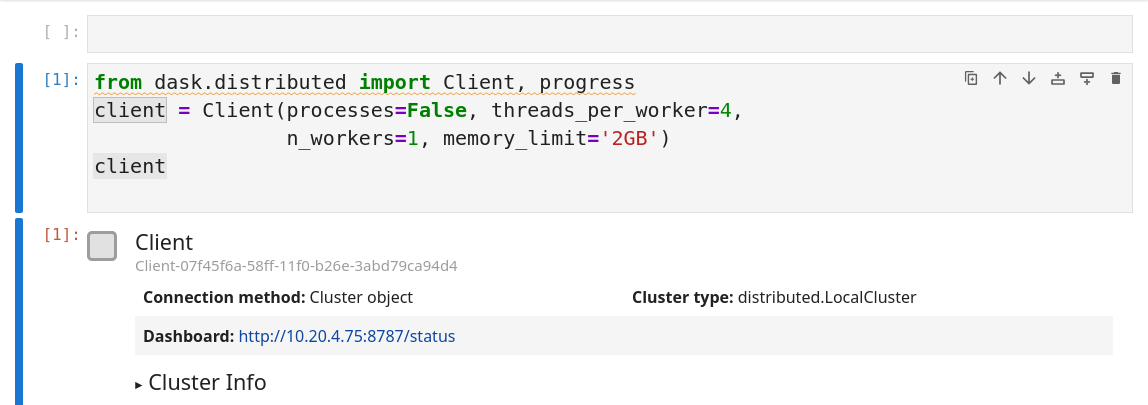
Using the Dask dashboard

In the information about the Dask cluster is a link to a Dashboard webpage. From the Dashboard we can monitor our Dask cluster and see how busy it is, view a graph of task dependencies, memory usage and the status of the Dask workers. This can be really useful when checking if our Dask cluster is behaving correctly and working out how optimally our code is making use of Dask’s parallelism. Note that it is not possible (or at least not without significant additional complexity) to access the Dask dashboard when running on the JASMIN notebook service.

Dask dashboard graph view

Dask dashboard task view

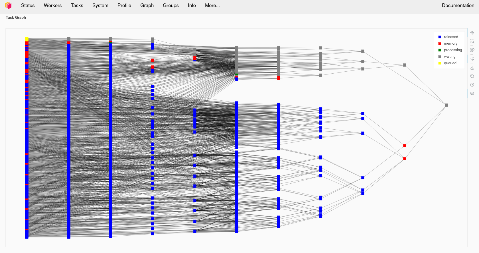
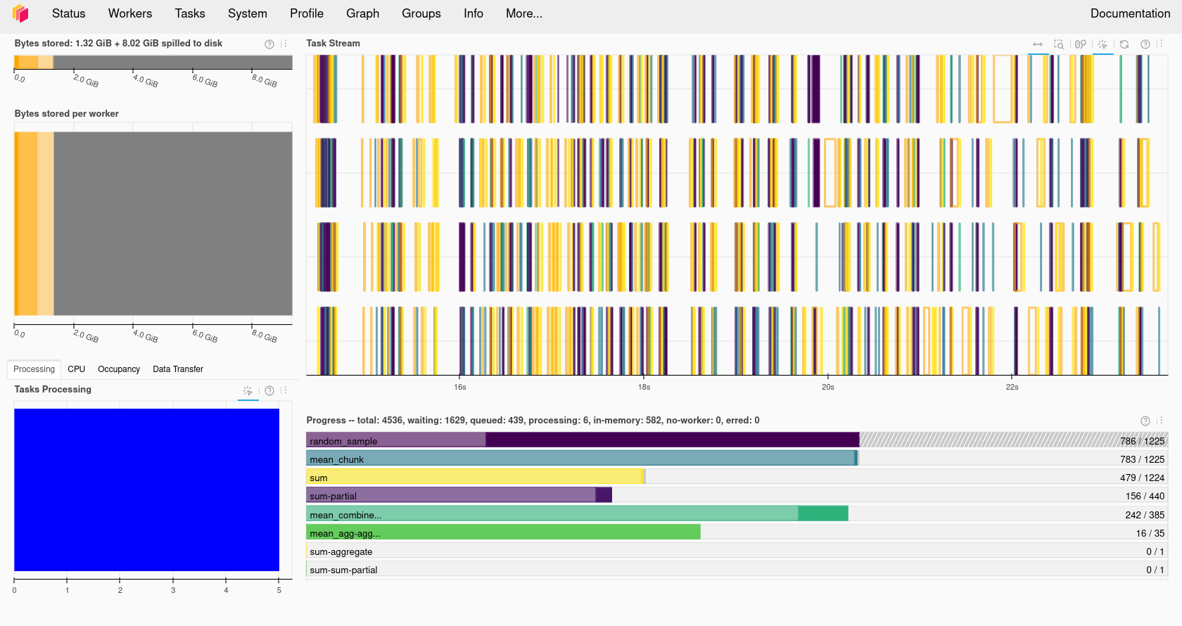
Using the JASMIN Dask gateway

JASMIN offers a Dask Gateway service which can submit Dask jobs to a special queue on the HPC cluster. To use this we need to do a bit of extra setup. We will need to import the dask_gateway library and configure the gateway.

PYTHON

import dask_gateway
gw = dask_gateway.Gateway("https://dask-gateway.jasmin.ac.uk", auth="jupyterhub")

The gateway can be given a set of options including how many worker cores to use, initially we can set this to one and scale it up later. We also need to allocate at least one core as to the scheduler which will manage our Dask cluster. JASMIN requires us to specify a project to associate the Dask jobs with. Users of training accounts should use “workshop”. Finally we need to tell Dask which Conda/Mamba environment to use and this needs to match the one we’re running in our notebook.

PYTHON

options = gw.cluster_options()
options.worker_cores = 1
options.scheduler_cores = 1
options.account = "workshop"
options.worker_setup='source /apps/jasmin/jaspy/miniforge_envs/jaspy3.11/mf3-23.11.0-0/bin/activate /work/scratch-nopw2/tobfer/cloud-native-geoscience-course-env'

Finally we can check if we already had a cluster running and reuse that if we do and then get a client object from the cluster that will behave the same way as the local Dask client did.

PYTHON

clusters = gw.list_clusters()
if not clusters:
    cluster = gw.new_cluster(options, shutdown_on_close=False)
else:
    cluster = gw.connect(clusters[0].name)

client = cluster.get_client()
client

Now that we have a running cluster we can allow it to adapt and scale up and down as we demand it. This will translate to jobs being launched on the JASMIN cluster itself. JASMIN allows users to spawn up to 16 jobs in the Dask queue, but one of these will be taken by the scheduler so we can only launch a maximum of 15 workers.

PYTHON

cluster.adapt(minimum=1, maximum=15)

Once we are done with Dask we can shutdown the cluster by calling its shutdown function. This should cause the jobs in the SLURM queue to finish.

PYTHON

cluster.shutdown()

With a Dask cluster running using dask_gateway you can now see the dashboard by clicking on the link in the client object.

Dask arrays and lazy computation

Dask arrays are chunked arrays that mimic NumPy’s API but execute lazily and in parallel. Any processing operations can work in parallel across these chunks. Data can also be loaded “lazily” into Dask Arrays, this means it is only loaded from disk when it is accessed. This can give us the illusion of loading a dataset that is larger than our memory.

Example:

PYTHON

import dask.array as da

# Create a 10000x10000 array of random numbers, chunked 1000x1000
x = da.random.random((10000, 10000), chunks=(1000, 1000))
print(x)

Simple operation: add ones

PYTHON

y = da.ones((10000, 10000), chunks=(1000, 1000))
z = x + y
print(z)  # Still a Dask array, not yet computed

As you can see, the addition operation does not compute the result immediately. Instead, it builds a task graph that describes how to compute z from x and y. The actual computation happens when you call .compute():

PYTHON

# Trigger computation
result = z.mean().compute()
print("Mean value:", result)

The new variable result will now contain the result of the computation and will be of the type numpy.ndarray.

PYTHON

type(result)

Important points:

• Creating x and y defines a Dask array with specified chunking, but no data is computed until needed.
• Operations build a task graph. .compute() runs the tasks.
• Chunking lets Dask process different blocks in parallel and only load chunks into memory when required.

Discussion

Exercise 1 - Compare Dask and NumPy performance

Compare the performance of the following code using Numpy and Dask functions. Use the %%time magic in the cells to find out the execution time. Ensure you only time the core computation and not the Dask cluster setup or library imports, this means you’ll have to write this code into multiple cells. Dask version (note you’ll need to do the Dask client setup first):

PYTHON

# Dask version
import dask.array as da
x = da.random.random((20000,20000), chunks=(1000,1000))
x_mean = x.mean()
x_mean.compute()

Numpy version:

PYTHON

import numpy as np
npx = np.random.random((20000,20000))
npx_mean = npx.mean()

Which went faster overall? Why do you think you got the result you did? Try making the dataset a little larger, going much beyond 25000x25000 might use too much memory. Try running the top command in a terminal while your notebook is running, look at the CPU % when running the Numpy and Dask versions and compare them. Try changing the number of Dask threads and see what effect this has on the CPU %.

To see the CPU % in a terminal you can use the command top or htop.

Checklist

Troubleshooting Dask

Sometimes Dask can jam up and stop executing tasks. If this happens try the following:

• Shutdown the client and restart it.
• Shutdown the kernel of your notebook and rerun the notebook.

Caution

Some pitfalls to watch out for

Combining lazy loading with parallel processing can be tricky. It is difficult to know when the data are actually being read from disk or downloaded from a remote source. This can lead to unexpected memory usage or performance issues.

So, when do the download and processing actually happen? Things that are usually obvious but catch us all off guard!

When you open a Zarr dataset with xarray, the data are not read into memory. The data are only read when you access them (e.g., by slicing or computing a statistic).

Dask with Zarr via xarray

---

The most common pattern in this workshop is to open a Zarr store with xarray and ask xarray to use Dask-backed chunks. Xarray then keeps the data lazy until you compute something.

First, create the client:

PYTHON

import xarray as xr
from dask.distributed import Client

client = Client(n_workers=2, threads_per_worker=2, memory_limit="1GB")
client

Then open the Zarr dataset with chunking:

PYTHON

base_path = "/gws/ssde/j25b/atlantis_vis/cloud-native-geoscience-course/" # or "" if you have the data in your current working directory

ds = xr.open_zarr(f"{base_path}data/era5_sst/ocean_temperature.zarr", chunks={})
print(ds)

sst = ds["sst"]
print(sst)

Because this dataset is already chunked, xarray can use the existing chunking from the Zarr store. In this case, you can set the chunks argument to {} or don’t specify it at all. Xarray will use the chunking from the Zarr store.

If you are using a netCDF dataset, to integrate Dask you would need to specify the chunk sizes when opening the dataset. For example:

PYTHON

ds_nc = xr.open_dataset(f"{base_path}data/era5_sst/ocean_temperature.nc", chunks={"valid_time": 10, "latitude": 100, "longitude": 100})

A simple parallel computation

PYTHON

corrected = sst * 1.1 - 1.0
global_mean = corrected.mean(dim=("latitude", "longitude"))
result = global_mean.compute()
print(result)

This workflow is important because the data stay lazy until .compute() is called. At that point Dask schedules the work across the chunks.

Challenge

Exercise 1 - Dask and xarray together

Using the zarr (data/era5_sst/ocean_temperature.zarr) dataset and the netCDF (data/era5_sst/ocean_temperature.nc) dataset, try the following:

1. Open each one with xarray, using xr.open_zarr for the Zarr dataset and xr.open_dataset for the netCDF dataset.
2. Compute a spatial mean over latitude and longitude.
3. Call .compute() in the zarr case and compare the result with and without Dask-backed chunks. Try to calculate the time taken for each computation and compare the results. You can use the %%time magic command in a Jupyter notebook to time the execution of a cell.

Questions:

• How does the chunking affect the computation?
• How does the performance differ between the Zarr and netCDF datasets?

Show me the solution

For the Zarr dataset:

PYTHON

%%time
base_path = "/gws/ssde/j25b/atlantis_vis/cloud-native-geoscience-course/" # or "" if you have the data in your current working directory
ds_zarr = xr.open_zarr(f"{base_path}data/era5_sst/ocean_temperature.zarr")
sst_zarr = ds_zarr["sst"]
global_mean_zarr = sst_zarr.mean(dim=("latitude", "longitude"))
result_zarr = global_mean_zarr.compute()

For the netCDF dataset:

PYTHON

%%time
ds_nc = xr.open_dataset(f"{base_path}data/era5_sst/ocean_temperature.nc")
sst_nc = ds_nc["sst"]
result_nc = sst_nc.mean(dim=("latitude", "longitude"))

When you compute the spatial mean over latitude and longitude for the Zarr dataset with Dask, you should see a reduction in computation time compared to the netCDF dataset. The exact performance gain will depend on the size of the dataset and the chunking strategy used.

Xarray plus Dask gives them a lazy, chunk-aware workflow. The important link is that chunking from the storage lesson now becomes the basis for parallel computation.

Callout

Other ways to parallelise Zarr workflows

Dask is the main parallel tool in this lesson, but Python has other ways to run work in parallel. The best choice depends on whether the task is CPU-bound, I/O-bound, or already chunked.

Threads

Thread-based parallelism can help when the work spends time waiting on I/O, which happens when reading chunks from a Zarr store. Threads are often useful for data access and downloading, but they are less flexible than Dask for organising a whole analysis workflow.

Multiprocessing

Python’s built-in multiprocessing is useful for independent tasks that do not need to share much state. It can work well for embarrassingly parallel jobs, but it is usually less convenient than Dask for Zarr and xarray because it does not understand chunks, task graphs, or labelled arrays automatically.

Cubed

Cubed is a library for chunked, out-of-core array processing. It is designed for large array computations and can be a good fit when you want to process Zarr-like data in a memory-aware way, especially in cloud-oriented workflows.

Visualising the Task Graph

---

To see how Dask is scheduling work, you can visualise the task graph. This can help you understand how many tasks are being created and how they depend on each other.

PYTHON

import dask
import xarray as xr

ds = xr.open_zarr(f"{base_path}data/era5_sst/ocean_temperature.zarr")
sst = ds["sst"]
corrected = sst * 1.1 - 1.0
global_mean = corrected.mean(dim=("latitude", "longitude"))
dask.visualize(global_mean, filename='task_graph.png')

Sometimes the visualize() function fails to find the path of graphviz, the library it uses to build the visualisation. If this is happening then run the following to fix it. Replace “/work/scratch-nopw2/tobfer/cloud-native-geoscience-course-env/bin/” with the path of the bin directory in your Conda/Mamba environment if you aren’t using the JASMIN environment.

PYTHON

import os
os.environ['PATH'] = "/work/scratch-nopw2/tobfer/cloud-native-geoscience-course-env/bin/:" + os.environ['PATH']

This will create a PNG file showing the task graph for the computation. You can also use global_mean.visualize() to see the graph directly in a Jupyter notebook.

Dask task graph

Challenge

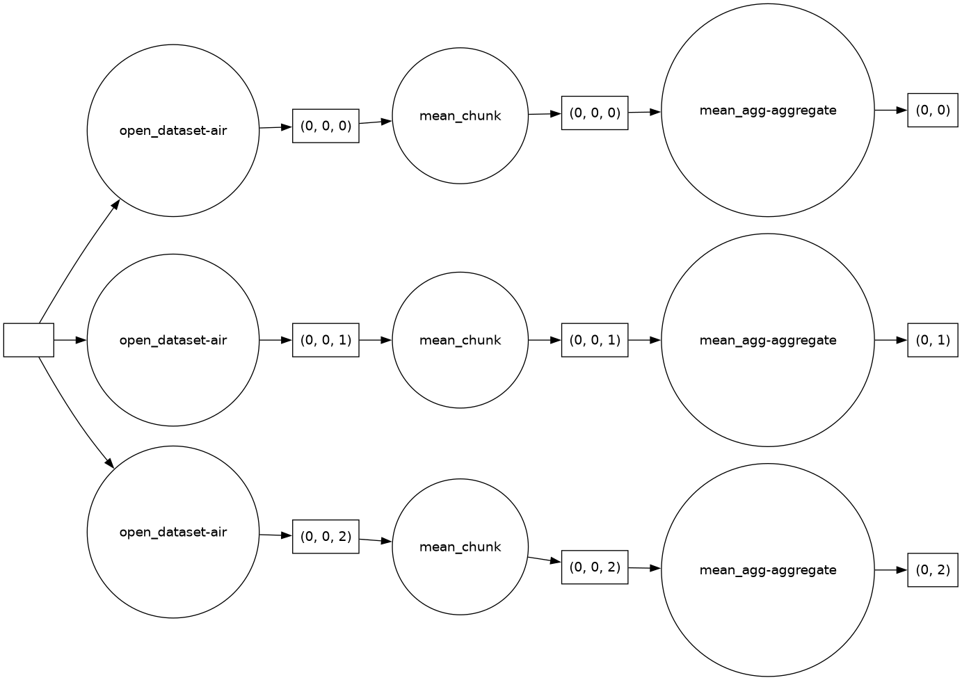
Exercise 2 - A small parallel workflow

Now, we are going to compare the results with different chunk sizes. Using the original zarr (data/era5_sst/ocean_temperature.zarr) and the rechunked zarr (data/era5_sst/ocean_temperature_rechunked.zarr - you created this in the previous episode) datasets, try the following:

1. Open the dataset
2. Run one spatial statistic and one time-based statistic.

For example (but you can choose any statistic you like):

PYTHON

# Spatial statistic: mean over latitude and longitude
spatial_mean = sst.mean(dim=("latitude", "longitude"))
# Time-based statistic: mean over time
time_mean = sst.mean(dim="time")

3. Repeat the same operation for the other dataset (the one you didn’t use in step 1).
4. Compare which version creates a more efficient task structure and which one runs faster. You can use the %%time magic command in a Jupyter notebook to time the execution of a cell.

Questions:

• Which dimensions matter most for your workflow?
• Did the chunk layout help or hurt parallel execution?
• How might the answer change if the data were much larger?

Show me the solution

For the original zarr dataset:

PYTHON

import xarray as xr

# Open the original zarr dataset
ds_original = xr.open_zarr(f"{base_path}data/era5_sst/ocean_temperature.zarr")
sst_original = ds_original["sst"]
# Spatial statistic: mean over latitude and longitude
spatial_mean_original = sst_original.mean(dim=("latitude", "longitude"))
# Time-based statistic: mean over time
time_mean_original = sst_original.mean(dim="valid_time")

%time spatial_mean_original.compute()
%time time_mean_original.compute()

For the rechunked zarr dataset:

PYTHON

# Open the rechunked zarr dataset
ds_rechunked = xr.open_zarr("data/era5_sst/ocean_temperature_rechunked.zarr")
sst_rechunked = ds_rechunked["sst"]
# Spatial statistic: mean over latitude and longitude
spatial_mean_rechunked = sst_rechunked.mean(dim=("latitude", "longitude"))
# Time-based statistic: mean over time
time_mean_rechunked = sst_rechunked.mean(dim="valid_time")
%time spatial_mean_rechunked.compute()
%time time_mean_rechunked.compute()

When you compute the spatial and time-based statistics for both the original and rechunked datasets, you should observe differences in execution time. The chunk layout can significantly affect parallel execution, especially for larger datasets.

Challenge

Exercise 3 (Optional) - Parallel workflow using a Dask cluster on HPC

Now we are going to explore how to run a parallel workflow using a Dask cluster on an HPC system like JASMIN. For this example, we are going to use a bigger dataset, the subset of the GLORYS Reanalysis dataset, stored in a single Zarr group (data/glorys/glorys_202605.zarr). This dataset is too large to process efficiently on a single core, so we will use Dask to parallelise the computation.

Please follow the steps below:

1. Set up a Dask cluster on JASMIN using the Dask Gateway service.
2. Open the GLORYS u-component of the ocean current velocity (uo) with Xarray.
3. Run a correction algorithm on the uo data (for example, multiply by a factor and subtract an offset). For example corrected_uo = uo * 1.1 - 1.0.
4. Experiment with:

• Changing the number of worker cores
• Changing the number of workers (set in cluster.adapt)

Show me the solution

Create a Dask cluster on JASMIN using the Dask Gateway service. You can use the following code snippet to set up the cluster and connect to it:

PYTHON

import dask_gateway
import xarray as xr

# Create a connection to dask-gateway.
gw = dask_gateway.Gateway("https://dask-gateway.jasmin.ac.uk", auth="jupyterhub")

options = gw.cluster_options()
options.worker_cores = 2
options.scheduler_cores = 1
options.account = "workshop"
options.worker_setup='source /apps/jasmin/jaspy/miniforge_envs/jaspy3.11/mf3-23.11.0-0/bin/activate /work/scratch-nopw2/tobfer/cloud-native-geoscience-course-env'
clusters = gw.list_clusters()
if not clusters:
    cluster = gw.new_cluster(options, shutdown_on_close=False)
else:
   cluster = gw.connect(clusters[0].name)

Now that we have a running cluster, we can get a client object from the cluster that will behave the same way as the local Dask client did.

PYTHON

client = cluster.get_client()
cluster.adapt(minimum=1, maximum=4)
ds = xr.open_zarr(f"{base_path}data/glorys/glorys_202605.zarr")
uo = ds['uo']
corrected_uo = uo * 1.1 - 1.0
corrected_uo.compute()
print(corrected_uo)

Remember to shutdown the cluster when you are done to free up resources:

PYTHON

cluster.shutdown()

Key Points

• “Dask is the main parallel tool used here.”
• “Zarr and Dask work well together because Zarr stores data in independent chunks.”
• “Xarray can open Zarr data lazily and hand chunked work to Dask.”
• “Other Python parallelism tools exist, but Dask is the most natural fit for chunked environmental data.”

Content from Reading Real-World Zarr Datasets in Python

---

Last updated on 2026-08-07 | Edit this page

Overview

Questions

• “Which publicly available Zarr datasets can I use for experimentation and learning?”
• “How do I open Zarr datasets from cloud object storage (Google Cloud, AWS S3) with Python?”
• “How do irregular grids, ragged arrays, and ensembles appear in Zarr + xarray?”
• “How do chunks and storage layout influence how I analyse these datasets?”

Objectives

• “Discover several open Zarr datasets for oceanography, climate, and meteorology.”
• “Use Python tools (xarray, zarr, fsspec) to open and explore Zarr datasets hosted in the cloud.”
• “Inspect dimensions, coordinates, and chunk layouts in real-world Zarr stores.”
• “Practice basic analysis and think about how chunking and storage affect performance.”

Overview: a tour of open Zarr datasets

---

In this lesson, we work hands‑on with several open Zarr datasets:

• IFS ensemble forecasts in Icechunk/Zarr from dynamical.org - global ensemble forecasts on AWS (Icechunk and its relationship to Zarr are explained later in this lesson).
• ERA5 ARCO reanalysis in Zarr on Climate Data Store - global atmospheric data ready for analysis.
• Sofar Spotter drifters - global Spotter wave drifter buoys from 2019-2023 stored as ragged array in Zarr.
• NEMO Near-Present-Day - global ocean multi-decadal Near-Present-Day simulations, developed by the National Oceanography Centre (NOC) in the UK.
• Additional examples such as CMIP6, CarbonPlan datasets and Earthmover Marketplace, depending on your interests.

Each dataset illustrates different aspects:

• Regular latitude-longitude grids.
• Ragged arrays (varying-length trajectories).
• Non-regular or irregular grids.
• Ensembles with member dimensions.

All these datasets are hosted in cloud object storage (Google Cloud, AWS S3, or HTTPS) and can be accessed programmatically with Python tools like xarray and zarr. Object storage and how it differs from traditional file systems are explained later in this lesson.

These datasets can be several terabytes in size. DO NOT DOWNLOAD THEM LOCALLY.

Ensemble forecasts - ECMWF AIFS ENS Icechunk/Zarr

---

Dynamical.org hosts ECMWF AIFS single and ensemble forecasts (ENS) in Icechunk/Zarr format on AWS S3. It is possible to access the data using the dynamical.org API or directly via the S3 url.

For example, the ECMWF AIFS SINGLE are accessible this way:

PYTHON

import xarray as xr

ds = xr.open_zarr("https://data.dynamical.org/ecmwf/aifs-single/forecast/latest.zarr")
ds

You can see as output that the dataset is large (14TB) and has dimensions for init_time, lead_time, latitude, and longitude. The data variables include various meteorological fields such as temperature, wind, and cloud cover.

If we inspect temperature_2m, we see that it represents hundreds of gigabytes of data:

PYTHON

ds['temperature_2m']

Let’s try and read it by slicing out a small part of the file. We will slice out the last initialisation time, and get all the lead_times and latitude and longitudes related to it:

PYTHON

temperature_2m = ds['temperature_2m'].isel(init_time=slice(-1, None))
temperature_2m

Now: - init_time is reduced to 1 - the selected time corresponds to the most recent model run (yesterday or today depending on the time of day)

This subset is much smaller, but no data has been loaded yet. If we explore further and print the temperature_2m array we’ll see that it is actually using a Dask array underneath.

PYTHON

print(temperature_2m)

To convert this into a standard Xarray DataArray we can call .compute() on the temperature_2m. Note that only now will the data be loaded into memory. This is a good example of lazy loading, where the data is not actually read until we explicitly ask for it.

PYTHON

temperature_2m_local = temperature_2m.compute()

We can now plot this by selecting the data for the first lead time and then plotting it (we also need to select the first initialisation time since we only have one):

PYTHON

temperature_2m_local.isel(init_time=0, lead_time=0).plot()

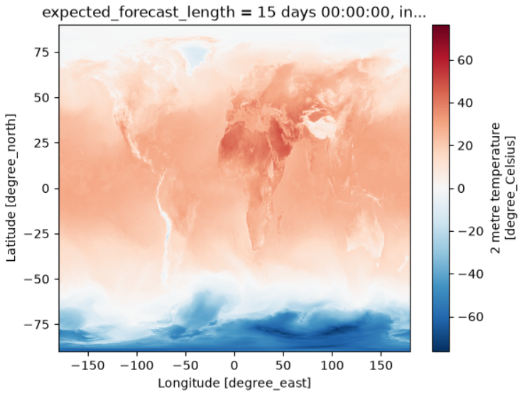
Or access some of the data:

PYTHON

temperature_2m_local[0,0,0,0].values

OUTPUT

array(0.15820312, dtype=float32)

If you want to slice the data by the latitude and longitude coordinates you can use sel instead of isel:

PYTHON

temperature_2m_slice = ds['temperature_2m'].sel(latitude=slice(50, 60), longitude=slice(-10, 0))
temperature_2m_slice

Exploring more datasets and examples

If you want to have access to more datasets, you can explore the dynamical.org catalog for other ECMWF datasets in Icechunk/Zarr format. You can also find some examples of how to access and manipulate these datasets in the dynamical.org documentation.

Callout

Integrate cartopy for better visualisation

The following example integrates cartopy to visualise the sea zonal wind at 10 meters above the surface from the ECMWF AIFS SINGLE dataset:

PYTHON

import xarray as xr
import matplotlib.pyplot as plt
import cartopy.crs as ccrs
import cartopy.feature as cfeature
ds = xr.open_zarr("https://data.dynamical.org/ecmwf/aifs-single/forecast/latest.zarr")
wind_u_10m = ds['wind_u_10m'].sel(init_time="2025-01-01",method="nearest").isel(lead_time=0)

plt.figure(figsize=(12, 6))
ax = plt.axes(projection=ccrs.PlateCarree())

# Add white land background
ax.add_feature(cfeature.LAND, facecolor='white', zorder=1)

ax.coastlines()
pcm = ax.pcolormesh(
    wind_u_10m.longitude, wind_u_10m.latitude, wind_u_10m,
    transform=ccrs.PlateCarree(),
    cmap="viridis",
    shading="auto",
    zorder=0  # Ensure it overlays the land
)

plt.title("Sea Zonal Wind at 10 Meters Above the Surface")
plt.colorbar(pcm, label=wind_u_10m.attrs.get("units", ""))
plt.tight_layout()
plt.show()

ERA5 ARCO - global reanalysis in Zarr

---

A subset of the ERA5 single-levels dataset is available in analysis-ready, cloud-optimised (ARCO) Zarr stores in the Copernicus Climate Data Store (CDS). The ARCO data is a repackaged version of the original ERA5 data. It allows direct programmatic access to a selection of the surface and wave variables (see below) without downloading individual files, enabling efficient and scalable data access and retrieval.

Create a CDS account and get an API key

1. Go to the Copernicus Climate Data Store and create an account.

2. After logging in, go to your API key page and copy your API key.

Access datasets

Set the cdsapi_key variable in the code below to your API key. This will allow you to access the ERA5 ARCO Zarr datasets hosted on the Copernicus Climate Data Store.

PYTHON

cdsapi_key = "<INSERT-CDS-API-KEY-HERE>"

For this example, we will use the wave dataset from the ERA5 ARCO dataset, which includes variables such as significant wave height (swh), mean wave period (mwp), and mean wave direction (mwd). The dataset is available in two chunking layouts: geo-chunked and time-chunked.

PYTHON

# Geo-chunked wave data (optimised for time-series at a single location)
geochunked_wav_url = "https://arco.datastores.ecmwf.int/cadl-arco-geo-003/arco/reanalysis_era5_single_levels/wav/geoChunked.zarr"

# Time-chunked wave data (optimised for global map at a single time step)
timechunked_wav_url = "https://arco.datastores.ecmwf.int/cadl-arco-time-003/arco/reanalysis_era5_single_levels/wav/timeChunked.zarr"

Let’s open the time-chunked dataset using xarray. Make sure to replace <INSERT-CDS-API-KEY-HERE> with your actual API key.

PYTHON

import xarray as xr

# Open the zarr store with xarray, users must insert their API key where indicated.
ds = xr.open_zarr(
    timechunked_wav_url,
    consolidated=True,
     storage_options = {
        "headers": {"Authorization": f"Bearer {cdsapi_key}"}
    }
)

# Inspect the variables
print(ds)

This is the output you should see:

OUTPUT

<xarray.Dataset> Size: 2TB
Dimensions:    (time: 758352, latitude: 361, longitude: 720)
Coordinates:
  * time       (time) datetime64[ns] 6MB 1940-01-01 ... 2026-07-05T23:00:00
  * latitude   (latitude) float64 3kB -90.0 -89.5 -89.0 -88.5 ... 89.0 89.5 90.0
  * longitude  (longitude) float64 6kB -180.0 -179.5 -179.0 ... 179.0 179.5
Data variables:
    mwd        (time, latitude, longitude) float32 788GB dask.array<chunksize=(1, 361, 720), meta=np.ndarray>
    mwp        (time, latitude, longitude) float32 788GB dask.array<chunksize=(1, 361, 720), meta=np.ndarray>
    swh        (time, latitude, longitude) float32 788GB dask.array<chunksize=(1, 361, 720), meta=np.ndarray>
Attributes:
    Conventions:             CF-1.7
    GRIB_centre:             ecmf
    GRIB_centreDescription:  European Centre for Medium-Range Weather Forecasts
    GRIB_edition:            1
    GRIB_subCentre:          0
    history:                 2024-09-05T05:51 GRIB to CDM+CF via cfgrib-0.9.1...
    institution:             European Centre for Medium-Range Weather Forecasts

For a full list of available variables, see the ERA5 ARCO documentation.

Create a plot of a variable

The following example shows how to create a plot of the significant wave height (swh) variable at a single time step using matplotlib:

PYTHON

import matplotlib.pyplot as plt

# Select a variable (e.g. significant wave height)
swh = ds["swh"]  # adjust to match the dataset variable names

# Select a single time step
one_time = swh.sel(time="2000-01-01T00:00:00")

# Plot the variable
plt.figure(figsize=(12, 6))
one_time.plot(cmap="coolwarm")
plt.title("ERA5 Significant Wave Height on 2000-01-01")
plt.xlabel("Longitude")
plt.ylabel("Latitude")
plt.show()

You can also use the geo-chunked dataset to get a time series of a specific location and plot it. You can see an example below for the significant wave height (swh) variable at a specific latitude and longitude (Rio de Janeiro coast):

PYTHON

ds_geo = xr.open_zarr(
    geochunked_wav_url,
    consolidated=True,
     storage_options = {
        "headers": {"Authorization": f"Bearer {cdsapi_key}"}
    }
)
swh = ds_geo["swh"]

# Select a specific location (e.g. Rio de Janeiro coast)
swh = swh.sel(latitude=-23.0, longitude=-43.0, method="nearest")

# Plot the time series
swh.plot()

Additional resources

To see a full list of available datasets and examples, you can explore the Copernicus Climate Data Store and the ECMWF Training datasets repository.

Sofar Spotter drifters - ragged arrays

---

The Sofar Spotter Archive provides historical wave and inferred wind data from a global network of Spotter buoys, in both NetCDF and Zarr formats. A Spotter is a small, solar-powered drifter buoy that measures wave height, period, and direction, as well as GPS location. The Sofar Ocean company has deployed thousands of Spotters worldwide, and some of the data is made available for research and analysis.

Sofar Spotter drifters deployed by Brazilian Navy and INPE, in partnership with Sofar Ocean

Array of spotter buoys

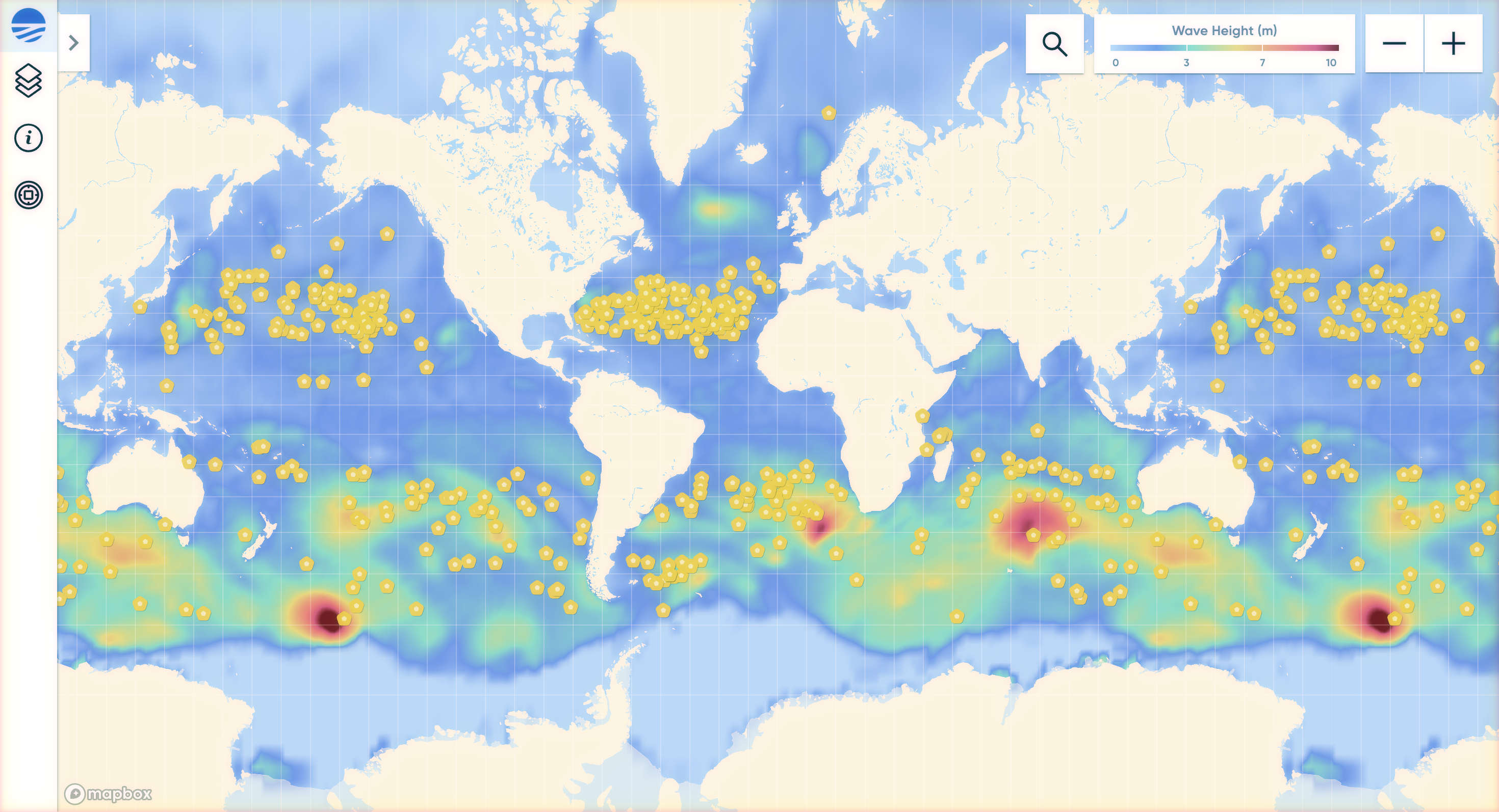
First, let’s open the Zarr dataset from the Sofar Spotter Archive using xarray. The dataset is hosted on AWS S3 and can be accessed directly via its URL:

PYTHON

import xarray as xr

s3_uri = "https://sofar-spotter-archive.s3.amazonaws.com/spotter_data_bulk_zarr"
ds = xr.open_zarr(s3_uri)
ds

OUTPUT

<xarray.Dataset> Size: 511MB
Dimensions:                (index: 6390651, trajectory: 871)
Coordinates:
    time                   (index) datetime64[ns] 51MB dask.array<chunksize=(99854,), meta=np.ndarray>
  * trajectory             (trajectory) object 7kB 'SPOT-010001' ... 'SPOT-1975'
Dimensions without coordinates: index
Data variables:
    latitude               (index) float64 51MB dask.array<chunksize=(99854,), meta=np.ndarray>
    longitude              (index) float64 51MB dask.array<chunksize=(99854,), meta=np.ndarray>
    meanDirection          (index) float64 51MB dask.array<chunksize=(99854,), meta=np.ndarray>
    meanDirectionalSpread  (index) float64 51MB dask.array<chunksize=(99854,), meta=np.ndarray>
    meanPeriod             (index) float64 51MB dask.array<chunksize=(99854,), meta=np.ndarray>
    peakDirection          (index) float64 51MB dask.array<chunksize=(99854,), meta=np.ndarray>
    peakDirectionalSpread  (index) float64 51MB dask.array<chunksize=(99854,), meta=np.ndarray>
    peakPeriod             (index) float64 51MB dask.array<chunksize=(99854,), meta=np.ndarray>
    rowsize                (trajectory) int64 7kB dask.array<chunksize=(871,), meta=np.ndarray>
    significantWaveHeight  (index) float64 51MB dask.array<chunksize=(99854,), meta=np.ndarray>
Attributes:
    author:         Isabel A. Houghton
    creation_date:  2023-10-18 00:43:55.333537
    email:          isabel.houghton@sofarocean.com
    institution:    Sofar Ocean
    references:     https://content.sofarocean.com/hubfs/Spotter%20product%20...
    source:         Spotter wave buoy
    title:          Sofar Spotter Data Archive - Bulk Wave Parameters

Dataset structure

This dataset was designed to follow the conventions used by NOAA for a similar dataset: Global Drifter Program (GDP) Drifter data. The explanation below about this dataset was extracted and adapted from the OHW 2024 Tutorials.

Each Spotter buoy records a different number of observations because of factors such as deployment time, reporting frequency, instrument lifetime, and missing measurements. One way to represent these observations is as an incomplete multidimensional array, where each column corresponds to a Spotter:

incomplete Array representation

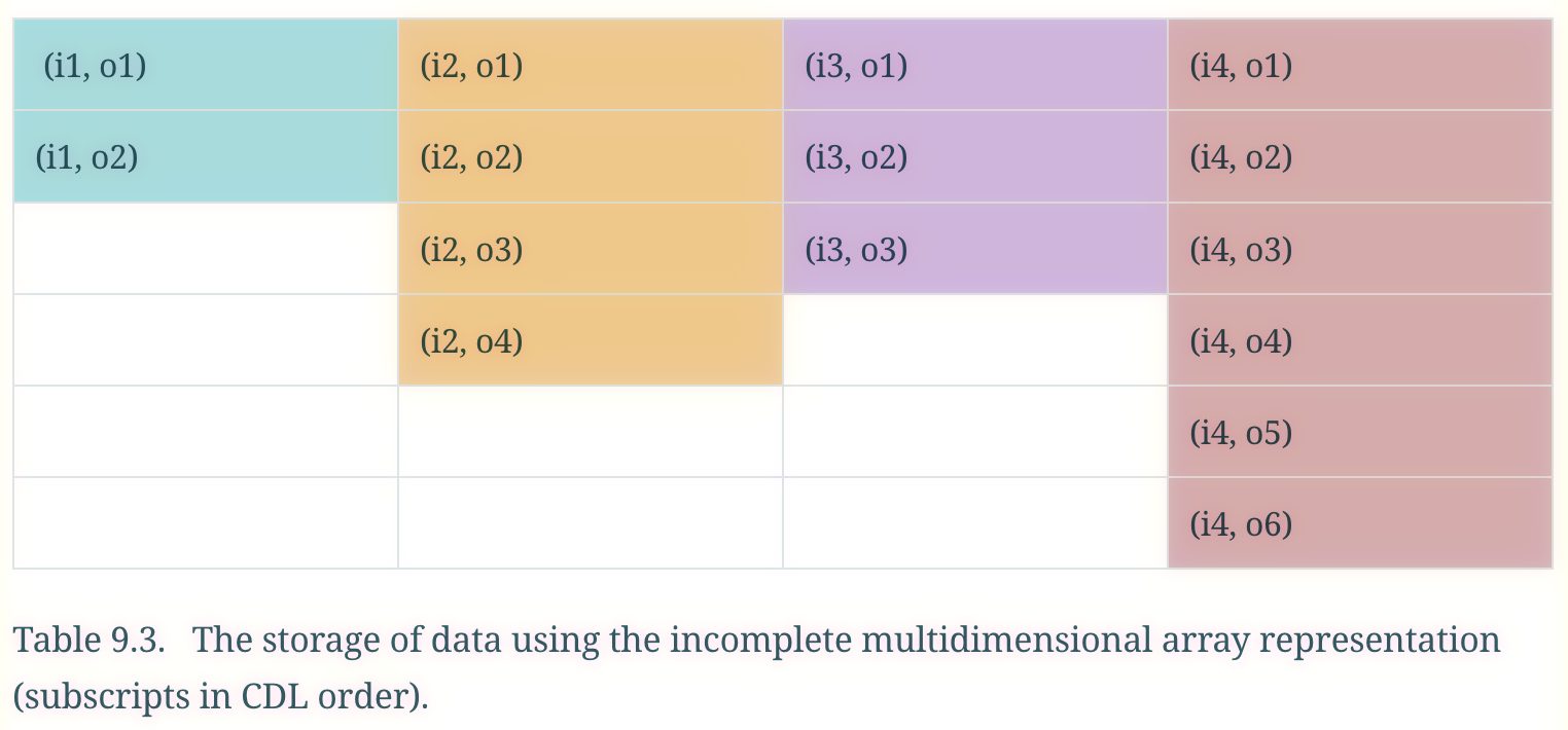
Although this representation is intuitive, it requires padding shorter time series with missing values. For large datasets, these unused values can occupy a substantial amount of storage. To avoid this overhead, the GDP and Sofar Spotter Archive use a contiguous ragged array representation:

Ragged array structure

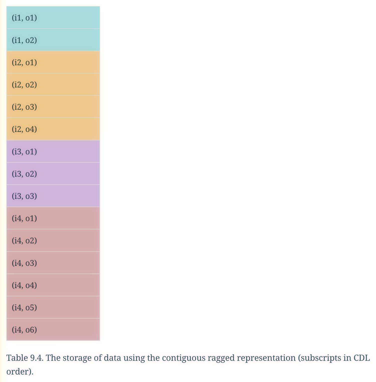
In a contiguous ragged array, observations from all Spotters are stored sequentially in a single array. Additional index variables identify which observations belong to each Spotter, eliminating the need to store missing values while preserving the original trajectories.

Plot drift trajectory for individual drifter colored by date

Get the data for a single drifter:

PYTHON

import numpy as np
# choose a drifter by ID
spotter_id = 'SPOT-0164'


# create array that points to indices for each trajectory
traj_idx = np.insert(np.cumsum(ds.rowsize.values), 0, 0)


# find index of chosen drifter
j = np.where(ds.trajectory==spotter_id)[0][0]
print(f"Drifter index for {spotter_id} is {j}")


# create the slice index `sli` for data from that drifter
sli = slice(traj_idx[j], traj_idx[j+1])

Plot the trajectory colored by significant wave height (swh):

PYTHON

import matplotlib.pyplot as plt
import cartopy.crs as ccrs
import xarray as xr

fig, ax = plt.subplots(
    figsize=(15, 10),
    subplot_kw={"projection": ccrs.PlateCarree()},
)

ax.coastlines()
ax.gridlines(draw_labels=True)
ax.set_extent([110, 260, -10, 60], crs=ccrs.PlateCarree())
# Convert longitudes to the [0, 360] range
lons = ds.longitude[sli].compute()
lons[lons<0] += 360 # make sure lons span [0,360] for easier mapping

sc = ax.scatter(
    lons,
    ds.latitude[sli],
    c=ds.significantWaveHeight[sli],
    s=12,
    cmap="viridis",
    transform=ccrs.PlateCarree(),
)

plt.colorbar(
    sc,
    ax=ax,
    label="Significant Wave Height (m)",
    shrink=0.3,
    pad=0.08,
)

ax.set_title(f"Trajectory of {spotter_id} colored by Significant Wave Height")

plt.show()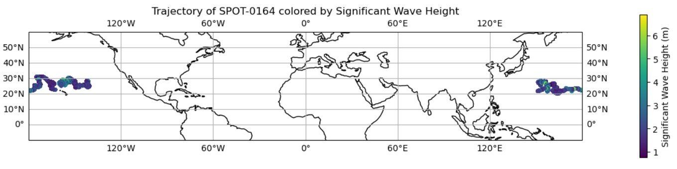

Trajectory of SPOT-0164

NEMO Near-Present-Day simulations

---

The NOC Near-Present-Day (NPD) simulations are multi-decadal global ocean and sea-ice simulations produced with NEMO. They include a hierarchy of model configurations at nominal resolutions of 1 degree, 1/4 degree, and 1/12 degree. The outputs are kept close to the present day and are made available through NOC’s cloud data catalog. The data is stored in Icechunk format (we will talk more about it later).

NOC created a python package called OceanDataStore to facilitate access to the NPD simulations and other datasets. The package provides a simple interface to search and open datasets from the catalog, which is built on top of STAC (SpatioTemporal Asset Catalog) metadata.

The OceanDataStore API lets us search the catalog by metadata rather than needing to know a Zarr store URL. In this example, we find annual output containing sea surface temperature:

PYTHON

from OceanDataStore import OceanDataCatalog
catalog = OceanDataCatalog(catalog_name="noc-stac") # open the catalog "noc-stac" from NOC's STAC server

# Search for datasets in the catalog with specific metadata
catalog.search(
    collection="noc-npd-era5",
    standard_name="sea_surface_temperature",
)

Now, let’s open the first item in the catalog only for the years 1980-1990:

PYTHON

ds_npd = catalog.open_dataset(
    id=catalog.available_items[0],
    start_datetime="1980-01",
    end_datetime="1990-12",
)

With the dataset open, you can plot the time mean:

PYTHON

ds_npd["tos_con"].mean(dim="time_counter").plot(cmap="RdBu_r")

See the full OceanDataCatalog example to explore other model resolutions, variables, pre-calculated diagnostics, and model-domain data.

Challenge

Exercise 1 - ECMWF AIFS SINGLE

Assuming you have opened an AIFS single dataset:

1. Identify the dimensions and coordinates of the dataset (e.g. init_time, lead_time, latitude, longitude).
2. Choose a variable (e.g. temperature_2m or similar, depending on the dataset’s naming).
3. Compute:

• A global mean time series over a limited period (e.g. one week).
• A spatial map at a single time step.

Show me the solution

PYTHON

import xarray as xr
import numpy as np
# Open the AIFS single dataset
ds = xr.open_zarr("https://data.dynamical.org/ecmwf/aifs-single/forecast/latest.zarr")

# Inspect dimensions and coordinates
print(ds.dims)
print(ds.coords)

# Choose a variable
temp = ds["temperature_2m"]  # adjust to match the dataset variable names

# Subset to one week (e.g. first week of the latest init_time)
temp_week = temp.isel(init_time=-1).sel(lead_time=slice(np.timedelta64(0, "D"), np.timedelta64(7, "D")))

# Global mean time series
global_ts = temp_week.mean(dim=("latitude", "longitude"))
print(global_ts)

# Map at a single time step (e.g. first lead_time of the week)
one_time = temp_week.isel(lead_time=0)
one_time.plot()

Challenge

Exercise 2 - Climate Data Store ERA5 inspection and simple analysis

1. First, ensure you have your CDS API key set up as described above.
2. Inspect the ERA5 dataset:
   • Print era5.dims, era5.data_vars, and era5.coords.
   • Identify at least 2 variables of interest (e.g. mwp, swh).
3. Select one variable (e.g. mwp for mean wave period) and subset it to a specific time range (e.g. one year).
4. Compute:
   • A global mean time series over a limited period (e.g. one year).
   • A spatial map at a single time step.

Show me the solution

PYTHON

import xarray as xr

cdsapi_key = "<INSERT-CDS-API-KEY-HERE>"
# Open the ERA5 dataset
era5 = xr.open_zarr(
    "https://arco.datastores.ecmwf.int/cadl-arco-time-003/arco/reanalysis_era5_single_levels/wav/timeChunked.zarr",
    consolidated=True,
    storage_options={"headers": {"Authorization": f"Bearer {cdsapi_key}"}}
)

# Inspect dimensions, data variables, and coordinates
print(era5.dims)
print(era5.data_vars)
print(era5.coords)

# Select a variable (e.g. mean wave period)
mwp = era5["mwp"]  # adjust to match the dataset variable names

# Subset to a specific time range (e.g. one year)
mwp_year = mwp.sel(time=slice("2020-01-01", "2020-12-31"))

# Global mean time series
global_ts = mwp_year.mean(dim=("latitude", "longitude"))
print(global_ts)

# Spatial map at a single time step (e.g. first time step of the year)
one_time = mwp_year.isel(time=0)
one_time.plot()

Challenge

Exercise 3 - Working with ragged arrays

1. Open the Sofar Spotter drifter dataset as shown above.
2. Inspect ds_spot:
   • Print ds_spot.dims, ds_spot.coords, and ds_spot.data_vars.
   • Identify the ragged structure: which dimensions represent trajectories, which represent sample indices?
3. Choose one trajectory (e.g. trajectory="SPOT-010001" or similar) and extract its time series:
4. Plot a time series of a variable of interest (e.g. significantWaveHeight) for that trajectory.

Show me the solution

PYTHON

import xarray as xr

# Open the Sofar Spotter drifter dataset
s3_uri = "https://sofar-spotter-archive.s3.amazonaws.com/spotter_data_bulk_zarr"
ds_spot = xr.open_zarr(s3_uri)

# Inspect dimensions, coordinates, and data variables
print(ds_spot.dims)
print(ds_spot.coords)
print(ds_spot.data_vars)

# Identify the ragged structure
# 'trajectory' dimension represents different drifters, 'index' represents sample indices
# Choose one trajectory and extract its time series
spotter_id = "SPOT-010001"
traj_idx = np.insert(np.cumsum(ds_spot.rowsize.values), 0, 0)
j = np.where(ds_spot.trajectory == spotter_id)[0][0]
sli = slice(traj_idx[j], traj_idx[j + 1])

# Plot a time series of significant wave height for that trajectory
import matplotlib.pyplot as plt

plt.figure(figsize=(12, 6))
plt.plot(ds_spot.time[sli], ds_spot.significantWaveHeight[sli])
plt.title(f"Significant Wave Height for {spotter_id}")
plt.xlabel("Time")
plt.ylabel("Significant Wave Height (m)")
plt.grid()
plt.show()

Challenge

Exercise 4 - Exploring the Near-Present-Day simulations

1. Create an OceanDataCatalog and search the noc-npd-era5 collection for sea_surface_temperature.
2. Inspect catalog.available_items and identify the item for annual 1-degree eORCA1 output.
3. Open the item for 2000-2010 and inspect its dimensions, variables, and chunking.
4. Plot the mean sea surface temperature over this period. Remember that the catalog returns lazy data: avoid loading the complete simulation.

Show me the solution

PYTHON

from OceanDataStore import OceanDataCatalog

catalog = OceanDataCatalog(catalog_name="noc-stac")
catalog.search(
    collection="noc-npd-era5",
    standard_name="sea_surface_temperature",
)
print(catalog.available_items)

ds_npd = catalog.open_dataset(
    id="noc-npd-era5/npd-eorca1-era5v1/r1i1c1f1/gn/T1y",
    start_datetime="2000-01",
    end_datetime="2010-12",
)

print(ds_npd.dims)
print(ds_npd.data_vars)
print(ds_npd["tos_con"].chunks)

ds_npd["tos_con"].mean(dim="time_counter").plot(cmap="RdBu_r")

Other open Zarr datasets to explore

---

You can broaden the lesson with other open Zarr datasets:

• CMIP6 Zarr on AWS - global climate model output in Zarr format in the AWS open data.
• CarbonPlan Zarr datasets - downscaled climate and other datasets accessible via HTTPS-friendly Zarr URLs.
• Earthmover Marketplace - a collection of open geoscience datasets, some of which are available in Zarr format.

Discussion

Exercise 5 (Optional) - Build your own mini project

Choose one of the datasets (ERA5, Spotter, AIFS, CMIP6, NEMO, or another Zarr dataset you know) and design a mini project:

1. Define a question you want to answer (e.g. “How has near‑surface temperature changed in a region over a given period?” or “What is the distribution of wave heights across the Spotter network?”).
2. Write code to:
   • Open the dataset with xarray and/or supporting libraries.
   • Explore dimensions, variables, chunk strategy and metadata.
   • Perform a small analysis or visualisation that addresses your question.
3. Reflect on:
   • How easy or difficult it was to access and manipulate the Zarr dataset.
   • How chunks and storage affected performance and workflow.
   • Any issues or surprises you encountered (e.g. irregular grids, ragged arrays, ensemble dimensions).

You can share your mini projects with the class or colleagues and discuss different approaches.

Key Points

• “Many open Zarr datasets are available for oceanography, climate, and meteorology, including ERA5 ARCO, Sofar Spotter drifters, ECMWF IFS ensemble forecasts, CMIP6, and marine products.”
• “Python tools like xarray, zarr, and fsspec make it straightforward to open and explore Zarr datasets hosted on cloud object storage.”
• “Real-world Zarr datasets illustrate regular grids, ragged arrays, ensemble dimensions, and more, providing rich practice for accessing, analysing, and understanding chunked data.”
• “Working hands-on with open Zarr datasets helps learners build intuition about data structures, performance, and best practices for cloud-native scientific workflows.”

Content from Object Storage and Cloud Data Organization

---

Last updated on 2026-08-10 | Edit this page

Overview

Questions

• “What is an object store, and how is it different from storing data on a server filesystem?”
• “Why is object storage a good fit for large-scale data sharing and cloud-native science?”
• “How does object storage support secure, concurrent, and parallel access?”
• “How can I use commercial cloud object stores and self-hosted solutions like MinIO?”

Objectives

• “Explain what object storage is and how it differs from traditional file and block storage.”
• “Describe why object storage is useful for sharing, durability, and parallel access.”
• “Understand how to access cloud object stores (S3, GCS, Azure Blob) from Python.”
• “Deploy a simple self-hosted S3-compatible object store (MinIO) using Docker.”

What is object storage?

---

Object storage stores data as objects in a flat address space, usually inside buckets. Each object contains binary data and metadata (such as content type or custom tags) and is identified by a unique key within a bucket, rather than by a path in a nested directory tree.

Unlike traditional storage systems:

• File storage (POSIX filesystems) organises data into directories and files.
• Block storage presents fixed-size blocks to an operating system and is commonly used for disks and databases.

Object storage is designed for storing large collections of independent objects that are accessed through APIs such as HTTP or S3. This architecture enables systems to scale across many disks and nodes while providing high durability.

Object storage and traditional servers

Traditional scientific workflows often store data on local or network filesystems:

• Data are stored in directories on one server or a small cluster.
• Access is provided through SSH, NFS, or mounted drives.
• Storage capacity and bandwidth are limited by the underlying hardware.

Object storage takes a different approach:

• Data are distributed across many disks and nodes, often spanning multiple availability zones or data centres.
• Applications access data through standard APIs, such as Amazon S3, Google Cloud Storage (GCS), or Azure Blob Storage.
• Storage systems can grow incrementally by adding new nodes rather than replacing existing hardware.

For scientific datasets, this makes it practical to store millions of independent objects, such as NetCDF files, image tiles, or Zarr chunks. Because each object can be accessed independently, applications running on HPC systems, cloud platforms, or local infrastructure can efficiently process data in parallel while accessing the same shared dataset.

Source

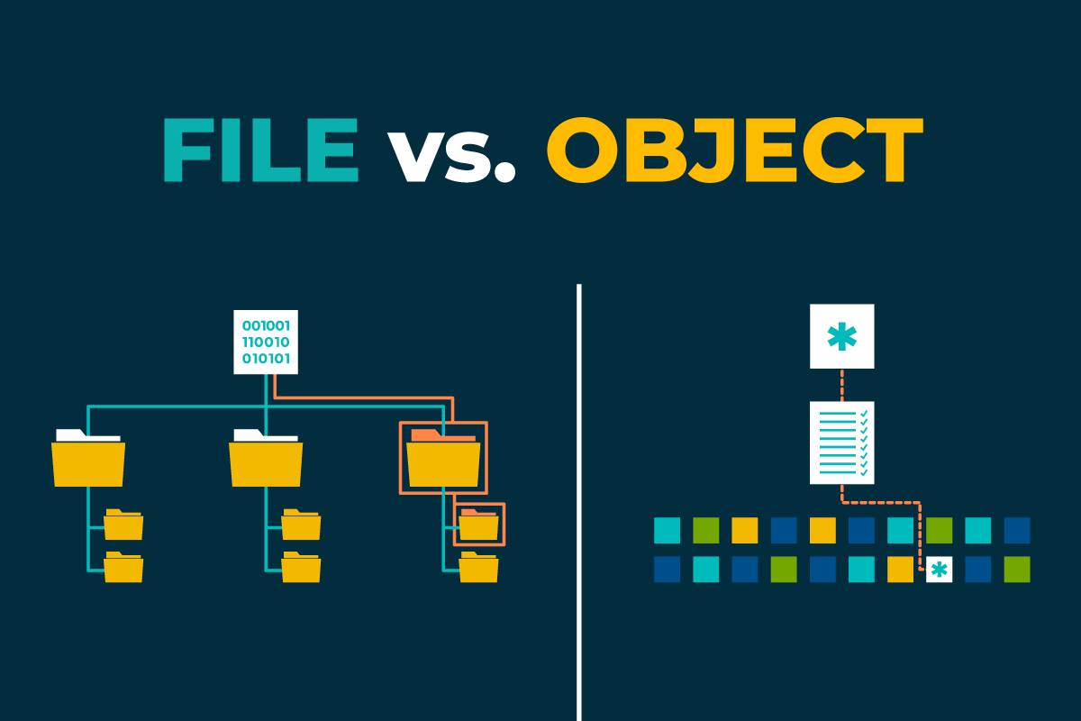
Advantages of object storage

---

Sharing and durability

Object storage is well suited for sharing and long-term preservation because it provides:

• Global access through URLs or API endpoints.
• Fine-grained access control using bucket policies, access control lists (ACLs), identity management, or signed URLs.
• High durability through replication or erasure coding across multiple disks and nodes.
• Support for per-object metadata, versioning, and public or private buckets.

Cloud Object Storage Architecture

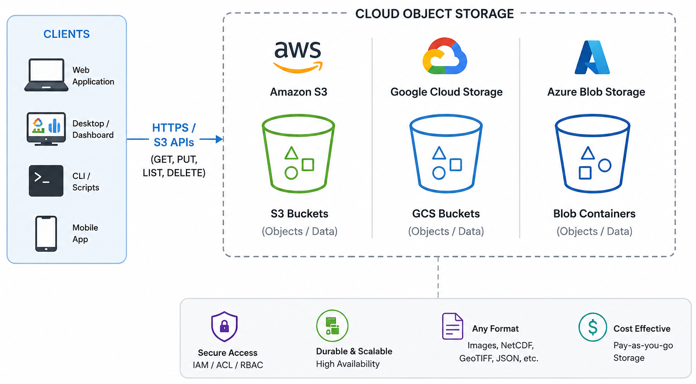
Security and access control

Object stores provide several layers of security:

• Authentication verifies the identity of users or services through access keys, OAuth tokens, or service identities.
• Authorisation controls who can read, write, list, or manage objects using policies, roles, and ACLs.
• Encryption protects data both in transit and at rest, with some systems also supporting client-side encryption.

Parallel and concurrent access

Each object in an object store can be accessed independently. As a result:

• Multiple clients can read and write different objects simultaneously.
• Large datasets composed of many objects (such as Zarr chunks) can be processed in parallel.
• Requests are distributed across many servers and disks, increasing aggregate throughput.

Frameworks such as Dask, Spark, and Apache Beam take advantage of this model by assigning different objects or chunks to different workers. This is one reason why cloud-native formats such as Zarr are commonly paired with object storage.

Cost and storage classes

Cloud providers typically offer multiple storage classes for different access patterns:

• Frequent access: higher performance for data that are accessed regularly.
• Infrequent access: lower storage cost with higher retrieval charges.
• Archive (cold storage): lowest storage cost, but higher retrieval latency and fees.

Selecting the appropriate storage class helps balance cost and performance according to how often the data are used.

Discussion

Deployment trade-offs

There are several ways to deploy object storage:

• Traditional file servers: simple to operate for small groups but limited by local hardware.
• Cloud object storage: provides elastic capacity, managed infrastructure, and high durability, with costs based on storage, requests, and data transfer.
• Self-hosted object storage: allows institutions to use existing hardware while retaining control over their infrastructure, but requires ongoing management, monitoring, backups, and maintenance.

The best choice depends on factors such as dataset size, access patterns, operational expertise, and budget.

For large scientific archives, the key question is not only “what is cheapest per terabyte?”, but also “what is cheapest and safest over the full life of the data?”

All the advantages of object storage make it a good fit for scientific data workflows, especially when combined with chunked formats like Zarr. The ability to store many independent objects, access them in parallel, and manage them through APIs allows researchers to build scalable, reproducible, and shareable data systems.

Traditional workflows vs New workflows

Challenge

Exercise 1 - Compare storage options for a workflow

Imagine your group needs to store a 10 TB Zarr dataset that is read often by several researchers.

1. Decide whether the dataset would be better suited to:
   • a traditional server filesystem,
   • cloud object storage,
   • or a self-hosted object store.
2. Write down two reasons for your choice.
3. Consider the following:
   • How often the data are accessed.
   • Whether multiple users need concurrent access.
   • Whether the data need to stay inside an institution.
   • Whether the group has staff to operate storage infrastructure.

Questions:

• Which option would be easiest to scale?
• Which option would be easiest to share securely?
• Which option would be most difficult to maintain over time?

Show me the solution

The answer will depend on the specific context of the group and their requirements. For example: - If the dataset is accessed frequently by multiple researchers and needs to be shared securely, cloud object storage may be the best option due to its scalability and built-in access controls. - If the dataset must remain within the institution due to data sovereignty concerns, a self-hosted object store may be preferable, provided the institution has the necessary staff and infrastructure to maintain it. - If the dataset is small and accessed by a single researcher, a traditional server filesystem may suffice, but it may become difficult to scale and maintain over time.

Accessing cloud object storage from Python

---

Common cloud object stores include AWS S3, Google Cloud Storage (GCS), Azure Blob Storage, and S3-compatible services such Cloudflare and JASMIN. Each has its own API and client libraries, but they all support S3-style access.

In Python, different providers have different client libraries, but for scientific workflows the most common pattern is to use S3-style access through boto3, fsspec, or s3fs:

• boto3 for AWS S3 and S3-compatible services.
• fsspec / s3fs for opening remote filesystems from Python and xarray.
• gcsfs or provider-specific libraries for Google Cloud Storage.
• azure-storage-blob for Azure Blob.

In this lesson, we focus on S3-style access because it is widely supported and works well with Zarr and xarray. It is the same one that JASMIN and other HPC/cloud platforms use for object storage.

Listing objects

For listing data in the object store, we will focus on boto3 (AWS S3) and fsspec/s3fs (for xarray and Zarr).

First, let’s see how to list objects in a public bucket using boto3 in a public cloud object store. For this example, we will use the NOAA GOES-18 public bucket, which has data from the GOES-18 satellite. This bucket is public, which does not require credentials for reading objects.

The first step is to create the client.

PYTHON

import boto3
from botocore import UNSIGNED
from botocore.config import Config

s3 = boto3.client(
    "s3",
    config=Config(signature_version=UNSIGNED), # UNSIGNED allows public access without credentials
)

After creating the client, we can list objects in a bucket. For example, to list the first 10 objects in the noaa-goes18 bucket under the prefix ABI-L2-CMIPF/, we can use the following code:

PYTHON

response = s3.list_objects_v2(
    Bucket="noaa-goes18",
    Prefix="ABI-L2-CMIPF/",
    MaxKeys=10,
)

for obj in response.get("Contents", []):
    print(obj["Key"])

To access a protected bucket, like the course bucket, you first provide your credentials. In this workshop, the credentials were supplied by the instructor. As we are using JASMIN, we also need to specify the endpoint URL for the S3-compatible service.

The following example shows how to list objects in a private bucket using boto3 with credentials:

PYTHON

import boto3

s3 = boto3.client(
    "s3",
    endpoint_url="https://atlantis-vis-o.s3-ext.jc.rl.ac.uk",
    aws_access_key_id="your-access-key",
    aws_secret_access_key="your-secret-key",
)

bucket_name = "cloud-native-geoscience-course"

response = s3.list_objects_v2(Bucket=bucket_name, MaxKeys=10)

for obj in response.get("Contents", []):
    print(obj["Key"], obj["Size"])

Once authenticated, you can list objects, inspect prefixes, and identify Zarr stores that you want to open later with xarray or zarr.

Callout

Bucket policy

The bucket used in this workshop allows public read access to objects, so files can be opened without AWS credentials if you already know the object path. For discovery and bucket listing, however, the workshop provides read-only credentials so participants can browse the bucket contents without being able to modify anything.

The bucket is configured with a policy similar to the example below:

JSON

{
  "Version": "2012-10-17",
  "Statement": [
    {
      "Effect": "Allow",
      "Principal": "*",
      "Action": [
        "s3:GetObject",
        "s3:ListBucket"
      ],
      "Resource": [
        "arn:aws:s3:::my-bucket",
        "arn:aws:s3:::my-bucket/*"
      ]
    }
  ]
}

This approach provides a simple and secure way to share datasets with a group of users. Participants can discover and read data without requiring full access to the bucket or individual AWS accounts.

Challenge

Exercise 2 - Access the course bucket with credentials

In this exercise, use the course credentials to connect to the object store we are using in this workshop.

1. Load the credentials provided by the instructor into your Python environment.
2. Use boto3 to list a few objects in the course bucket.

Questions:

• What prefixes or object names can you see?
• How does the organisation of the bucket reflect the data structure?
• How does accessing the bucket with credentials compare with mounting a filesystem?

Show me the solution

To access the course bucket, you can use the following Python code snippet. Make sure to replace "your-access-key" and "your-secret-key" with the actual credentials provided in the course materials.

PYTHON

import os
import boto3

os.environ["AWS_ACCESS_KEY_ID"] = "your-access-key"
os.environ["AWS_SECRET_ACCESS_KEY"] = "your-secret-key"

s3 = boto3.client("s3", endpoint_url="https://atlantis-vis-o.s3-ext.jc.rl.ac.uk")

bucket_name = "cloud-native-geoscience-course"
response = s3.list_objects_v2(Bucket=bucket_name)

for obj in response.get("Contents", []):
    print(obj["Key"], obj["Size"])

Authenticated access to object storage is straightforward in Python once the credentials are set. Bucket and key naming reflect the organisation of the data, such as by variable, time, or dataset.

Using xarray with a bucket

Assuming the credentials are already set, you can open a Zarr store directly with xarray once you know the bucket and object path:

PYTHON

import os
import xarray as xr

storage_options = {
    "key": os.environ["AWS_ACCESS_KEY_ID"],
    "secret": os.environ["AWS_SECRET_ACCESS_KEY"],
    "client_kwargs": {"endpoint_url": "https://atlantis-vis-o.s3-ext.jc.rl.ac.uk"},
    # these are JASMIN-specific options to avoid checksum errors on some datasets
    "config_kwargs": {
        "request_checksum_calculation": "when_required",
        "response_checksum_validation": "when_required",
    },
}

ds = xr.open_zarr(
    "s3://cloud-native-geoscience-course/ocean_temperature.zarr",
    storage_options=storage_options,
)

print(ds)

Once you know the bucket and object path, you can use the same pattern for other remote stores.

Because this bucket is public, you can also open the Zarr store without credentials (using the public endpoint) as follows:

PYTHON

ds = xr.open_zarr("https://atlantis-vis-o.s3-ext.jc.rl.ac.uk/cloud-native-geoscience-course/ocean_temperature.zarr")

Listing the bucket contents still requires the read-only credentials described above.

Challenge

Exercise 3 - Open a Zarr store from the course bucket

In the same object store that you explored in the previous exercise, now open a Zarr store with xarray and inspect its contents. Reuse the bucket listing from Exercise 2 to find a Zarr dataset different from ocean_temperature.zarr, then open that store and inspect its dimensions, variables, and metadata.

Show me the solution

Reuse the bucket listing from Exercise 2 to identify a Zarr store, for example glorys_202605.zarr. Then open it with xarray:

PYTHON

import xarray as xr
import os

storage_options = {
    "key": os.environ["AWS_ACCESS_KEY_ID"],
    "secret": os.environ["AWS_SECRET_ACCESS_KEY"],
    "client_kwargs": {"endpoint_url": "https://atlantis-vis-o.s3-ext.jc.rl.ac.uk"},
    # these are JASMIN-specific options to avoid checksum errors on some datasets
    "config_kwargs": {
        "request_checksum_calculation": "when_required",
        "response_checksum_validation": "when_required",
    },
}

ds = xr.open_zarr(
    "s3://cloud-native-geoscience-course/glorys_202605.zarr",
    storage_options=storage_options,
)

print(ds)

In this example, you will see the variables, dimensions, and shapes of the Zarr store. The key point is that object storage discovery and dataset analysis are separate steps: first find the store, then open it with xarray.

Self-hosted object storage

---

Some institutions cannot or do not want to place all data in a commercial cloud. Common reasons include data sovereignty, procurement rules, local security requirements, network bandwidth constraints, and the desire to keep very large datasets close to on-premise compute systems.

In those settings, self-hosted object storage can be a strong option. It gives you the S3-style API that modern scientific tools expect, while keeping the data inside your own infrastructure. This is especially useful for universities, research institutes, and government organisations that already run their own servers, storage, and clusters.

What infrastructure is needed locally?

A production-ready object store is more than “just a server with a disk”. For a high-speed and reliable deployment, institutions usually need:

• Multiple storage nodes, not a single machine.
• Fast networking, ideally 10/25/100 GbE depending on scale.
• Redundant disks, typically SSD or NVMe for higher throughput, or carefully planned HDD tiers for colder data.
• Enough memory and CPU to support erasure coding, metadata handling, and many concurrent requests.
• Separate backup and monitoring systems.
• Stable power, cooling, and physical security.
• A plan for identity, access control, and certificate management.

Callout

Minimal MinIO deployment with Docker Compose

In class, we will not expect you to run these commands yourself. Instead, we will show how a self-hosted S3-compatible service such as MinIO could be deployed inside an institution’s own infrastructure, so that you can see how the same tools and APIs work on-prem as well as in the cloud.

On a Linux server with Docker and Docker Compose installed:

Create a directory and a docker-compose.yml:

YAML

services:
  minio:
    image: minio/minio:latest
    container_name: minio
    ports:
      - "9000:9000"  # S3 API
      - "9001:9001"  # Web UI
    environment:
      MINIO_ROOT_USER: minioadmin
      MINIO_ROOT_PASSWORD: minioadmin123
    volumes:
      - /data:/data   # bind mount for data
    command: server /data --console-address ":9001"
    restart: unless-stopped

Start MinIO:

BASH

docker compose up -d

Then:

• Open the web console at http://localhost:9001.
• Log in with minioadmin / minioadmin123 (change these in production!).
• Create a bucket (e.g. example-bucket).
• Upload a test file.

You now have a self-hosted S3-compatible object store. You can use standard S3 tools (e.g. AWS CLI, boto3, mc MinIO client) to interact with this bucket, just pointing them at your MinIO endpoint (http://localhost:9000).

Organising data in buckets and objects

---

Whether you use cloud or self-hosted object storage, you need a sensible organisation scheme. Typical patterns include:

• Per project or product bucket (e.g. era5-reanalysis, spotter-archive, ifs-ens-forecast).
• Hierarchical prefixes in object keys to represent logical structure, for example:
  • variable/time/region/chunk.zarr
  • year/month/day/file.nc
  • model/experiment/member/store.zarr

Design considerations:

• Make it easy to list all data for a given variable or time range.
• Align prefixes with common queries (e.g. model/experiment for CMIP6; instrument/trajectory for drifters).
• Avoid excessively deep or inconsistent naming. Object storage does not require directories, but prefixes mimic them.

For Zarr stores:

• Each store typically resides under a single prefix (path/to/store.zarr), containing nested JSON metadata and data chunk objects.
• You may create separate stores for different variables, domains, or time ranges depending on data volumes and workflows.

Challenge

Exercise 4 - Design a bucket layout

Imagine you are responsible for storing:

• A global reanalysis (regular grid).
• A network of drifter trajectories (ragged arrays).
• An ensemble prediction system (with member dimension).

Propose a bucket and object key layout that:

1. Makes it easy to find data for a given product, variable, and time range.
2. Supports storing Zarr stores for gridded data.
3. Accommodates ragged and ensemble data in a clear way.

Write your proposed naming scheme (bucket names and key patterns) and share it with the group.

Show me the solution

We can propose a bucket layout that reflects the structure of the datasets and their access patterns. Here are some example layouts:

• reanalysis/<variable>/<year>/<month>/store.zarr for gridded data.
• drifters/<platform>/<trajectory>/data.zarr for ragged data.
• ens/<model>/<run>/<member>/store.zarr for ensemble data.

They will gain practice in thinking about organisational schemes that work well with object storage’s flat namespace and prefix listing.

Key Points

• “Object storage stores data as objects with keys and metadata in buckets, accessed via HTTP/S3-style APIs rather than local filesystems.”
• “Cloud object stores (S3, GCS, Azure Blob, S3-compatible services) offer durable, scalable, and secure storage well suited to large scientific datasets.”
• “Parallel and concurrent access are natural in object storage, making it a good fit for chunked formats and distributed processing frameworks.”
• “Self-hosted object storage solutions like MinIO provide S3-compatible APIs and can be deployed with Docker on your own servers.”
• “Thoughtful bucket and key organisation is essential for efficient data discovery and workflow design in the cloud.”

Content from Converting Traditional Formats to Zarr

---

Last updated on 2026-08-05 | Edit this page

Overview

Questions

• “Why convert NetCDF data to Zarr, and what changes in the way we access and process data?”
• “How do we choose chunk sizes for Zarr when starting from NetCDF files?”
• “How can we use Dask and xarray to convert and write data to Zarr efficiently?”
• “How do we test that the converted data is usable and correct (e.g. computing mean values)?”

Objectives

• “Explain the main steps in converting NetCDF datasets to Zarr.”
• “Choose appropriate chunking strategies for the target Zarr dataset.”
• “Use xarray, Dask, and to_zarr to convert NetCDF to Zarr in parallel.”
• “Upload Zarr stores to object storage and verify basic analyses on the converted data.”

Why convert NetCDF to Zarr?

---

NetCDF is widely used for ocean, climate, and meteorological data and works well on local filesystems and HPC storage. However, as datasets grow and we move to cloud and parallel computing, Zarr offers several advantages:

• Chunked storage aligned with object stores and HTTP/S3 access.
• Easy parallel reads/writes of chunks by Dask or other frameworks.
• Flexible layout for large collections (many NetCDF files → one Zarr dataset).

Converting NetCDF to Zarr does not change the scientific content, but it changes how data is organised and accessed, enabling cloud-native workflows and more efficient analysis at scale.

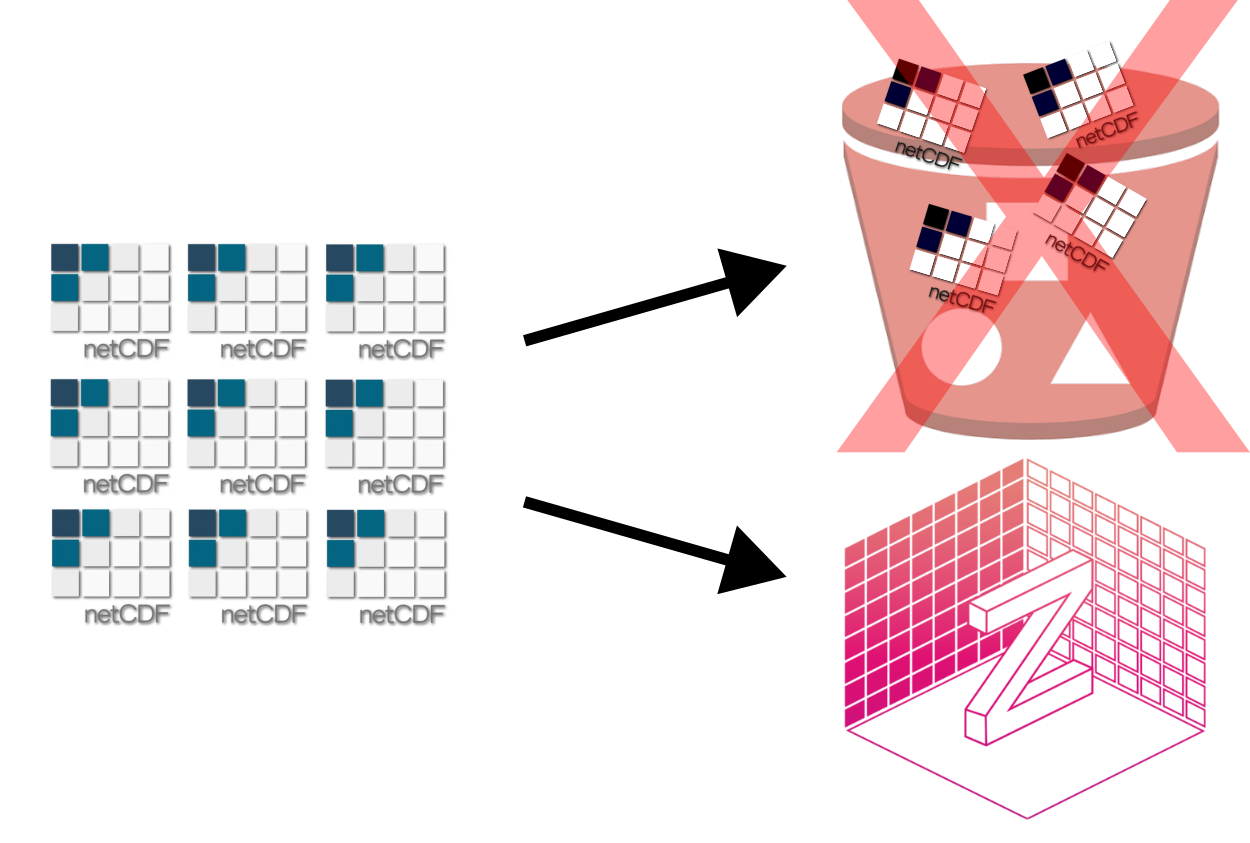
Converting from NetCDF to Zarr with xarray

To convert NetCDF to Zarr, we typically use xarray’s to_zarr method, optionally with Dask for parallelism. The following example uses the data/era5_sst/ocean_temperature.nc dataset:

1. Open data netCDF dataset with xarray:

PYTHON

import xarray as xr
base_path = "/gws/ssde/j25b/atlantis_vis/cloud-native-geoscience-course/" # or "" if you have the data in your current working directory
ds_nc = xr.open_dataset(f"{base_path}data/era5_sst/ocean_temperature.nc")
print(ds_nc)

2. Decide how the dataset should be chunked

The chunking scheme should match the way the data will be used later. A simple example chunking choice might look like this:

PYTHON

ds_nc = ds_nc.chunk({"valid_time": 10, "latitude": 100, "longitude": 100})
print(ds_nc.chunks)

3. Write the Zarr store

Once the chunking looks right, write the dataset to Zarr.

PYTHON

ds_nc.to_zarr("data/example.zarr", mode="w")

Now you have a local Zarr store that can be uploaded to object storage and accessed in parallel by multiple clients:

PYTHON

ds_zarr = xr.open_zarr("data/example.zarr")
print(ds_zarr)

Challenge

Exercise 1 - Convert a NetCDF dataset to Zarr

Using the NetCDF dataset provided (data/era5_sst/ocean_temperature.nc), open a single file with open_dataset, chunk it with {"valid_time": 10, "latitude": 100, "longitude": 100}, and write it to a local Zarr store.

Then, reopen the Zarr store and verify that the dimensions and variables match the original NetCDF dataset, and if the chunking is as expected.

Show me the solution

PYTHON

import xarray as xr

base_path = "/gws/ssde/j25b/atlantis_vis/cloud-native-geoscience-course/" # or "" if you have the data in your current working directory

ds_nc = xr.open_dataset(f"{base_path}data/era5_sst/ocean_temperature.nc")
ds_nc = ds_nc.chunk({"valid_time": 10, "latitude": 100, "longitude": 100})
ds_nc.to_zarr("data/example.zarr", mode="w")

PYTHON

ds_zarr = xr.open_zarr("data/example.zarr")
print(ds_zarr)

Overall workflow: NetCDF → Zarr → object store

---

In the real world, the conversion of NetCDF to Zarr is often done in a workflow that includes the following typical steps:

1. Understand the NetCDF input: check variables, dimensions, coordinates, and chunking.
2. Decide chunking strategy for Zarr: based on expected access patterns and approximate chunk sizes in MB.
3. Open NetCDF with xarray: using open_dataset or open_mfdataset for multiple files.
4. Apply chunking and encoding: use .chunk() and define any compression or encoding options.
5. (Optional) Write Zarr to local storage: using Dataset.to_zarr(), possibly with Dask for parallel writes.
6. Upload Zarr store to object storage: using cloud CLI tools or filesystem libraries, or directly write to object storage with fsspec.
7. Verify by reopening from object storage and running analyses (e.g. computing mean values).

We’ll walk through these steps conceptually and via exercises. For the example below, we will use a subset of the GLORYS Reanalysis dataset. The data is located in the data/glorys/ directory and is provided as multiple NetCDF files, one per day. The goal is to convert this collection of NetCDF files into a single Zarr store that can be accessed efficiently in parallel.

NetCDF-to-Zarr conversion should include chunk design, validation, and publishing checkpoints.

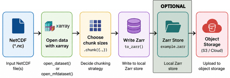
Step 1 - Inspect NetCDF inputs

---

Before converting, inspect the NetCDF file(s) you plan to convert.

Example of opening a single NetCDF file:

PYTHON

import xarray as xr

ds_nc = xr.open_dataset(f"{base_path}data/glorys/glorys_20260501.nc")
print(ds_nc)
print(ds_nc.dims)
print(ds_nc.data_vars)
print(ds_nc.coords)
print(ds_nc.encoding)  # may show chunking and compression info

Questions to answer:

• Are there multiple files (e.g. one per time slice) or just a single file?
• Which dimensions are present (e.g. time, lat, lon, depth, member)?
• Are variables chunked already, and if so, how?
• Are all files consistent in terms of variables and coordinates if you plan to use open_mfdataset?

Because we have multiple NetCDF files, we can use open_mfdataset to open them all at once:

PYTHON

ds_nc_multi = xr.open_mfdataset(
    f"{base_path}data/glorys/*.nc",
    combine="by_coords",
)
print(ds_nc_multi)

It is important to mention that open_mfdataset will combine multiple files into a single xarray dataset, but it requires that the variables and coordinates are consistent across files. And we are not loading the data into memory yet. Xarray will lazily load data as needed.

Step 2 - Decide chunking strategy for Zarr

---

Chunks in Zarr have a major impact on performance. A common rule of thumb is to aim for compressed chunk sizes in the range of 10-100 MB, but exact choices depend on workloads and hardware.

Consider:

• Dimensions: which ones correspond to time, space, depth, ensemble member?
• Workloads: time series at points, spatial means, regional subsets, ensemble statistics.
• Storage: local HPC disk vs object store, network bandwidth, parallel framework (Dask).

Example chunk strategy for a dataset with dimensions (time, latitude, longitude, depth):

• If time series are common: {"time": 360, "latitude": 100, "longitude": 100, "depth": 1}.
• If spatial maps per time are common: {"time": 1, "latitude": 361, "longitude": 720, "depth": 1}.
• If depth slices are common: {"time": 1, "latitude": 100, "longitude": 100, "depth": 10}.

You can experiment with different chunk shapes and use Dask’s dashboard and performance measurements to refine choices.

Step 3 - Convert NetCDF to Zarr with xarray and Dask

---

Once chunking decisions are made, you can use xarray’s to_zarr method to write out the dataset. This can be done serially or in parallel using Dask. For large datasets, parallel writing is often necessary to avoid long runtimes.

First, create a Dask client to manage parallelism:

PYTHON

from dask.distributed import Client
import xarray as xr

client = Client(n_workers=2, threads_per_worker=2)

Then, open the NetCDF dataset and apply chunking:

PYTHON

ds_nc = xr.open_mfdataset(f"{base_path}data/glorys/*.nc", combine="by_coords")

# Choose chunking
ds_chunked = ds_nc.chunk({"time": 5, "latitude": 400, "longitude": 400, "depth": 10})

Now you can write the chunked dataset to Zarr. You can choose to consolidate metadata for faster reads later:

PYTHON

ds_chunked.to_zarr("data/glorys.zarr", mode="w", consolidated=True)

Open the Zarr store to verify:

PYTHON

ds_zarr = xr.open_zarr("data/glorys.zarr", consolidated=True)
print(ds_zarr)

Callout

Consolidated metadata

When writing a Zarr store, you can choose to consolidate metadata. This means the store writes a single metadata index file, that collects the metadata for all arrays and attributes in one place.

This is useful because opening the dataset can be faster, especially when the store has many variables or many chunks. Instead of reading lots of small metadata files one by one, xarray can read the consolidated metadata in a single step.

A good practice is to use consolidated metadata when the dataset will be read many times after writing, especially in cloud or object-store workflows. It is usually a good default for analysis-ready Zarr stores.

Callout

Encoding and compression

When writing Zarr stores, you can choose how each variable is encoded and compressed. In most teaching and analysis workflows, the goal is not to maximise compression at all costs, but to choose a strategy that balances file size, speed, and ease of reading.

A simple example looks like this:

PYTHON

import zarr
from zarr.codecs import BloscCodec, BloscShuffle
import xarray as xr

ds = xr.open_dataset(f"{base_path}data/era5_sst/ocean_temperature.nc")
compressor = BloscCodec(cname="zstd", clevel=3, shuffle=BloscShuffle.shuffle)
encoding = {
    "sst": {
        "compressors": compressor,
        "chunks": (10, 100, 100),
    }
}

ds.to_zarr(
    "data/example_compressed.zarr",
    mode="w",
    encoding=encoding,
    consolidated=True,
)

In this example: - zstd gives good compression with reasonable speed. - clevel=3 is a moderate compression level, which is often a good compromise between speed and size. - shuffle=2 usually improves compression for many numerical datasets. - The same compressor is applied to each data variable through the encoding dictionary.

For scientific data, moderate compression is often a good default because it reduces storage size, lower network transfer costs, and keeps read/write speeds reasonable. Very aggressive compression can save more space, but it may slow down writing and reading. For large workflows, that trade-off is often not worth it.

Step 4 - Upload Zarr to object storage

---

After successfully writing Zarr locally, you can upload the Zarr directory store to an object store (AWS S3, GCS, MinIO, etc.).

The following example uses s3cmd, which is a command-line tool for interacting with S3-compatible object stores. You can also use other tools like awscli, rclone, or Python libraries like boto3 or fsspec.

BASH

# Create a bucket (if it doesn't exist)
s3cmd mb s3://my-bucket

# Upload the Zarr store recursively
s3cmd put -r data/glorys.zarr s3://my-bucket/glorys.zarr

Once uploaded, you can access the Zarr store directly from the object store using xarray and filesystem adapters, as in previous lessons.

In our lesson here, instead of generating the zarr dataset locally and upload then later to the object store, we will directly write the zarr dataset to the object store using fsspec. This is a more efficient approach and avoids unnecessary local storage usage. In the code below, remember to replace my-bucket with the actual bucket name you have access to (please ask the instructor for the bucket name and credentials).

Because the dataset is large, we will use the JASMIN dask cluster to run the conversion and upload, as it has better network access to the object store. You can see an example below, but you can also take a look in the Parallel Processing for Zarr episode for more details.

Create a connection to dask-gateway and start a cluster:

PYTHON

import dask_gateway

# Create a connection to dask-gateway.
gw = dask_gateway.Gateway("https://dask-gateway.jasmin.ac.uk", auth="jupyterhub")

options = gw.cluster_options()
options.worker_cores = 4
options.scheduler_cores = 2
options.account = "workshop"
options.worker_setup='source /apps/jasmin/jaspy/miniforge_envs/jaspy3.11/mf3-23.11.0-0/bin/activate /work/scratch-nopw2/tobfer/cloud-native-geoscience-course'
clusters = gw.list_clusters()
if not clusters:
    cluster = gw.new_cluster(options, shutdown_on_close=False)
else:
   cluster = gw.connect(clusters[0].name)
client = cluster.get_client()
cluster.adapt(minimum=1, maximum=4)

Create a mapper for the object store:

PYTHON

import xarray as xr
import fsspec
import os

store_url = "s3://my-bucket/glorys.zarr"

# remember to set the AWS_ACCESS_KEY_ID and AWS_SECRET_ACCESS_KEY environment variables with your credentials
os.environ["AWS_ACCESS_KEY_ID"] = "your-access-key"
os.environ["AWS_SECRET_ACCESS_KEY"] = "your-secret-key"

storage_options = {
    "key": os.environ["AWS_ACCESS_KEY_ID"],
    "secret": os.environ["AWS_SECRET_ACCESS_KEY"],
    "client_kwargs": {"endpoint_url": "https://atlantis-vis-o.s3-ext.jc.rl.ac.uk"},
    # The `config_kwargs` is required for JASMIN S3 object store.
    "config_kwargs": {
        "request_checksum_calculation": "when_required",
        "response_checksum_validation": "when_required",
    },
}

# Create a mapper for the object store
mapper = fsspec.get_mapper(
    store_url,
    **storage_options,
)

Write the dataset directly to the object store:

PYTHON

ds_chunked.to_zarr(
    mapper,
    mode="w",
    consolidated=True,
)

Step 5 - Verify with a simple analysis

---

To verify that the converted Zarr dataset is usable, run a simple analysis, such as computing a mean value. Example:

PYTHON

import xarray as xr
import fsspec

# Replace `my-bucket` with the actual bucket name you have access to.
mapper = fsspec.get_mapper(
    store_url,
    **storage_options,
)
ds_zarr = xr.open_zarr(mapper, consolidated=True)

# You can also access the dataset directly, as it is in a public bucket (replace with your own bucket if needed):
ds_zarr = xr.open_zarr("https://atlantis-vis-o.s3-ext.jc.rl.ac.uk/my-bucket/glorys.zarr", consolidated=True)

# Choose a variable
var = ds_zarr["zos"]

# Mean for each time step (global spatial mean)
mean_per_time = var.mean(dim=("latitude", "longitude")).compute()
print(mean_per_time)

# Mean for each latitude/longitude location (time mean)
mean_per_latlon = var.mean(dim="time").compute()
print(mean_per_latlon)

Challenge

Exercise 2 - Understand your NetCDF dataset

For the exercises 2-5, we are going to work with the subset of the ERA5 Reanalysis dataset related to the variable swh (significant wave height). The dataset is provided as multiple NetCDF files, one per day, in the data/daily_swh/ directory.

Using the NetCDF dataset(s) provided on the server:

1. Open a single file with open_dataset and print:
   • Dimensions and coordinates.
   • Data variables.
   • Encoding information (especially chunking).
2. Then, open multiple files with open_mfdataset and verify:
   • Consistency of variables and coordinates.
   • Combined time dimension length.

What are the main variables and dimensions you care about, and what is the existing chunking layout (if any)?

Show me the solution

Open a single NetCDF file:

PYTHON

import xarray as xr
ds_nc = xr.open_dataset(f"{base_path}data/daily_swh/swh_2025-01-01.nc")
print(ds_nc.dims)
print(ds_nc.data_vars)
print(ds_nc.coords)
print(ds_nc.encoding)

Open multiple NetCDF files:

PYTHON

ds_nc = xr.open_mfdataset(
    f"{base_path}data/daily_swh/swh_*.nc",
    combine="by_coords",
)
print(ds_nc.dims)
print(ds_nc.data_vars)
print(ds_nc.coords)

Now you should have a clear picture of the input data: variables, dimensions, coordinates, and any existing chunking or compression. This understanding is essential before deciding a Zarr chunk layout or doing any conversion.

Challenge

Exercise 3 - Propose Zarr chunk sizes

Based on your NetCDF dataset and expected workloads:

1. Propose a chunk dictionary, e.g. {"time": 720, "lat": 100, "lon": 100} or similar.
2. Estimate (roughly) the size of each chunk in bytes/MB (using variable sizes and dimension lengths).
3. Explain how your chunk choices support your intended analyses.

You do not need exact numbers. Focus on reasoning.

Show me the solution

PYTHON

# Example chunk proposal
chunking = {"time": 720, "latitude": 100, "longitude": 100}

chunk_size_bytes = (
    ds_nc["swh"].dtype.itemsize  # bytes per element
    * chunking["time"]
    * chunking["latitude"]
    * chunking["longitude"]
)
chunk_size_MB = chunk_size_bytes / (1024 ** 2)
print(f"Estimated chunk size: {chunk_size_MB:.2f} MB")

After calculating the estimated chunk size, you can reason about how this chunking supports your analysis:

PYTHON

ds_chunked = ds_nc.chunk(chunking)

You’d propose reasonable chunk sizes that reflect your workloads and aim for manageable chunk sizes. You will practice linking chunk shapes to analysis patterns, preparing for actual conversion.

Challenge

Exercise 4 - Convert your NetCDF dataset to Zarr in object storage

After opening and chunking the NetCDF dataset, convert it to Zarr and write it directly to the object store using fsspec.

Please use the credentials provided by the instructor to access the object store. For this exercise, use the JASMIN Dask cluster (or the local Cluster) to perform the conversion and upload, as it provides better network access to the object store. You can refer to the Parallel Processing for Zarr episode for more details.

Once the conversion is complete, reopen the dataset from the object store and verify that it can be read correctly.

Questions:

• How long did the conversion and upload take?
• Does the size of the Zarr store seem reasonable compared to the original NetCDF files?
• Were there any variables or attributes you needed to drop or adjust?
• Does the reopened dataset have the expected dimensions, variables, and attributes?

Show me the solution

First, create a Dask cluster and connect a client. You can use a local Cluster:

PYTHON

from dask.distributed import Client

client = Client(n_workers=2, threads_per_worker=2)

Or a JASMIN Dask cluster:

PYTHON

import dask_gateway

# Create a connection to dask-gateway.
gw = dask_gateway.Gateway(
    "https://dask-gateway.jasmin.ac.uk",
    auth="jupyterhub",
)

options = gw.cluster_options()
options.worker_cores = 2
options.scheduler_cores = 1
options.account = "workshop"
options.worker_setup = (
    "source /apps/jasmin/jaspy/miniforge_envs/jaspy3.11/"
    "mf3-23.11.0-0/bin/activate "
    "/work/scratch-nopw2/tobfer/cloud-native-geoscience-course"
)

clusters = gw.list_clusters()
if not clusters:
    cluster = gw.new_cluster(options, shutdown_on_close=False)
else:
    cluster = gw.connect(clusters[0].name)

client = cluster.get_client()
cluster.adapt(minimum=1, maximum=4)

Then convert the dataset directly to object storage and reopen it:

PYTHON

import os
import xarray as xr
import fsspec

storage_options = {
    "key": os.environ["AWS_ACCESS_KEY_ID"],
    "secret": os.environ["AWS_SECRET_ACCESS_KEY"],
    "client_kwargs": {
        "endpoint_url": "https://atlantis-vis-o.s3-ext.jc.rl.ac.uk",
    },
    "config_kwargs": {
        "request_checksum_calculation": "when_required",
        "response_checksum_validation": "when_required",
    },
}

store_url = "s3://my-bucket/era5_swh.zarr"
mapper = fsspec.get_mapper(
    store_url,
    **storage_options,
)

ds_chunked.to_zarr(
    mapper,
    mode="w",
    consolidated=True,
)

ds_zarr = xr.open_zarr(
    mapper,
    consolidated=True,
)

print(ds_zarr)

Writing directly to object storage avoids creating an intermediate local copy and reflects a typical cloud-native workflow. Reopening the dataset verifies that the conversion completed successfully and that the dataset structure and metadata have been preserved.

The time taken for conversion and upload will depend on the dataset size, chunking, network speed, and cluster resources. You can use Dask’s dashboard to monitor progress and performance.

Challenge

Exercise 5 - Check consistency and compute a mean

Using both the original NetCDF files dataset (ds_nc) and the converted Zarr dataset (ds_zarr from object storage):

1. Compute the same statistic in both cases (e.g. global mean temperature at a given time):
2. Compare the results for equality (or near-equality within floating point tolerance).
3. Compare the time taken to open the dataset and compute the statistic in both cases.

Show me the solution

PYTHON

import time

# NetCDF
t0 = time.time()
ds_nc = xr.open_mfdataset(f"{base_path}data/daily_swh/swh_*.nc", combine="by_coords")
var_nc = ds_nc["swh"]
# slice to a single time step for comparison
var_nc = var_nc.isel(time=0)
t1 = time.time()
mean_nc = var_nc.mean(dim=("latitude", "longitude"))

t2 = time.time()
print("NetCDF mean:", float(mean_nc.values))
print("Time to open NetCDF files:", t1 - t0, "seconds")
print("Time taken for NetCDF computation:", t2 - t1, "seconds")
print("Total time for NetCDF:", t2 - t0, "seconds")

# Zarr
t0 = time.time()
ds_zarr = xr.open_zarr("https://atlantis-vis-o.s3-ext.jc.rl.ac.uk/my-bucket/era5_swh.zarr", consolidated=True)
var_zarr = ds_zarr["swh"]
var_zarr = var_zarr.isel(time=0)
t1 = time.time()
mean_zarr = var_zarr.mean(dim=("latitude", "longitude"))
mean_zarr = mean_zarr.compute()
t2 = time.time()
print("Zarr mean:", float(mean_zarr.values))
print("Time to open Zarr store:", t1 - t0, "seconds")
print("Time taken for Zarr computation:", t2 - t1, "seconds")
print("Total time for Zarr:", t2 - t0, "seconds")

When done carefully, converting NetCDF to Zarr and back preserves scientific values. The mean values should match within floating point tolerance, confirming that the conversion workflow is valid.

Key Points

• “Converting NetCDF to Zarr enables cloud-native, chunked, and parallel-friendly access to large scientific datasets.”
• “Effective conversion requires understanding input data, choosing chunk sizes based on workloads, and using xarray’s to_zarr with appropriate encoding and compression.”
• “Dask can parallelise the conversion process, making it feasible to handle large collections of NetCDF files.”
• “Uploading Zarr stores to object storage allows distributed teams and tools to access the same datasets efficiently.”
• “Checking basic statistics (e.g. mean values) in NetCDF and Zarr versions helps verify that conversions preserve scientific content.”

Content from Case Studies

---

Last updated on 2026-08-05 | Edit this page

Overview

Questions

• “How are different teams and organisations actually converting and serving data in practice?”
• “What problems do they face, and which solutions have worked well (or badly)?”
• “What lessons can we take from their architectures and workflows for our own projects?”

Objectives

• “Hear real-world experiences from practitioners applying cloud‑native data workflows.”
• “Understand how different organisations approach data conversion, cataloguing, versioning, and visualisation.”
• “Reflect on how these examples inform your own architectural and best‑practice decisions.”

Session format

---

In this open session, invited speakers will briefly present their experience (e.g. 10-12 minutes each):

• Where they work and what kinds of data and applications they focus on.
• How they are converting and organising data (NetCDF → Zarr, virtual Zarr, STAC, GeoZarr, Icechunk, etc.).
• The main applications, users, and performance constraints they design for.
• Key architectural decisions, trade‑offs, and implications (governance, cost, reproducibility, operations).

After each talk, there will be a short Q&A, followed by a joint discussion at the end of the session.

Key Points

• “Real-world case studies show that cloud-native architectures differ by mission, user needs, scale, and operational constraints.”
• “Successful teams make explicit trade-offs among performance, cost, governance, reproducibility, and maintainability.”
• “Common building blocks include Zarr (physical or virtual), STAC for discovery, and versioning approaches for controlled updates.”
• “Architectural decisions should be guided by concrete workloads and user access patterns, not only by tool popularity.”
• “Cross-team sharing of implementation lessons helps avoid repeated mistakes and speeds up adoption of robust workflows.”

Content from Versioning Data with Icechunk

---

Last updated on 2026-08-05 | Edit this page

Overview

Questions

• “What problems arise when we use plain Zarr for shared, evolving datasets?”
• “How does Icechunk add safety, consistency, and reproducibility on top of Zarr?”
• “How can we use transactions to update data atomically and avoid partial writes?”
• “How can we reference and replay specific versions of data for reproducible analysis?”

Objectives

• “Explain why versioning is important for Zarr-based scientific datasets.”
• “Describe Icechunk’s core concepts: repositories, transactions, snapshots, branches, and tags.”
• “Use Icechunk with Zarr to perform atomic updates and create reproducible versions.”
• “Recover from mistakes and open specific versions of a dataset.”

Why data versioning matters

---

Zarr is a strong format for cloud and parallel data access, but by itself it does not provide transactions, version history, or a built-in way to recover from mistakes. That can be a problem for shared scientific datasets. If several people are updating data, readers may see incomplete changes, accidental overwrites can be hard to recover from, and analyses can become difficult to reproduce later.

Icechunk adds version control on top of Zarr. It lets you manage data in a repository with transactions, snapshots, branches, and tags, so you can update data atomically, recover from mistakes, and refer to exact versions in future analysis.

Source

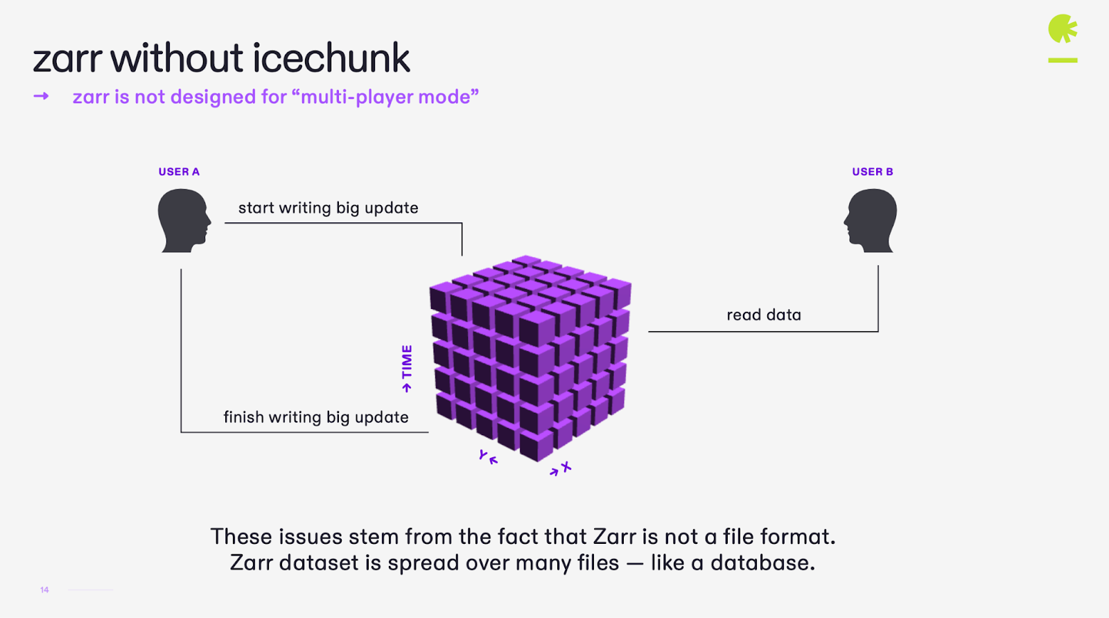
Icechunk concepts

---

Icechunk wraps Zarr stores inside repositories that track changes over time, in a similar way to how Git tracks changes to code. The main concepts are:

• Repository: the top-level object managing a Zarr hierarchy plus version history.
• Transaction: an atomic write session where multiple updates happen together; either all succeed or none do.
• Snapshot: an immutable version of the data after a transaction completes.
• Branch: a named line of development, such as main or dev.
• Tag: a human-readable label pointing to a specific snapshot, useful for reproducible references.

The main idea is simple: writes happen in transactions, commits create snapshots, and readers open read-only sessions that always see a complete version of the dataset.

Callout

Comparison of plain Zarr vs Icechunk

This example was adapted from the Earth Mover Github repository and shows how Icechunk adds versioning and transactional semantics to Zarr.

In the backend, we have a Zarr and an Icechunk repository that are being updated in a loop, following the same pattern.

If you try to read the plain zarr store while it is being updated, you will see a mix of old and new data:

PYTHON

import matplotlib.pyplot as plt
import zarr

store = zarr.storage.FsspecStore.from_url("https://atlantis-vis-o.s3-ext.jc.rl.ac.uk/icechunk-demo/zarr")
root = zarr.open_group(store=store, mode='r', zarr_format=3)
arr = root['image']
img_data = arr[:]

# Plot the data
plt.imshow(img_data)
plt.axis('off')
plt.show()

If you try to read the Icechunk store while it is being updated, you will see either the old snapshot or the new snapshot, but never a mix.

PYTHON

import matplotlib.pyplot as plt
import zarr
import icechunk as ic

storage = ic.s3_storage(
	bucket="icechunk-demo",
	prefix="icechunk",
	endpoint_url="https://atlantis-vis-o.s3-ext.jc.rl.ac.uk",
	anonymous=True,
	force_path_style=True,
)

ic_repo = ic.Repository.open(storage)

# Start a read-only icechunk session
session = ic_repo.readonly_session("main")

# Get the zarr store
store = session.store

# Get all the zarr array values
root = zarr.open_group(store=store, mode='r')
arr = root['image']
img_data = arr[:]

# Plot the data
plt.imshow(img_data)
plt.axis('off')
plt.show()

This shows that Icechunk provides a safe, consistent, and reproducible way to manage evolving Zarr datasets, making it suitable for collaborative scientific workflows.

Challenge

Exercise 1 - Map Git concepts to Icechunk

Before writing any code:

1. Map familiar Git concepts to Icechunk:
   • Git repository → Icechunk repository.
   • Git commit → Icechunk snapshot.
   • Git branch → Icechunk branch.
   • Git tag → Icechunk tag.
2. Discuss how these concepts help you reason about data changes over time.
3. Discuss how “time travel” supports reproducibility.

Show me the solution

Git concepts map naturally to Icechunk. An Icechunk repository stores the history of a dataset, similar to a Git repository for code. Snapshots are like Git commits, branches allow independent development, and tags mark important dataset versions.

These concepts make it easy to track changes, experiment safely, and understand how data evolves. Icechunk’s time travel feature allows you to access previous snapshots, making analyses reproducible by ensuring the exact dataset version can always be revisited.

Basic Icechunk workflow

---

A common workflow with Icechunk is:

1. Configure access to your object store.
2. Create or open an Icechunk repository in that object store.
3. Start a writable session on a branch such as main.
4. Add data to the repository, either by writing a dataset directly or by creating a virtual layer over an existing Zarr store.
5. Commit the session to create a snapshot.
6. Open the repository again in read-only mode for analysis.

In this lesson, we start with a Zarr dataset stored on your local machine and create an Icechunk repository in an object store. Once imported, the dataset can be versioned, allowing you to track changes over time while keeping the repository in object storage.

Step 1 - Connecting to the object store

PYTHON

import os
import xarray as xr
import icechunk as ic

os.environ["AWS_ACCESS_KEY_ID"] = "your-access-key"
os.environ["AWS_SECRET_ACCESS_KEY"] = "your-secret-key"

storage_options = {
    "key": os.environ["AWS_ACCESS_KEY_ID"],
    "secret": os.environ["AWS_SECRET_ACCESS_KEY"],
    "client_kwargs": {
        "endpoint_url": "https://atlantis-vis-o.s3-ext.jc.rl.ac.uk"
    },
    "config_kwargs": {
        "request_checksum_calculation": "when_required",
        "response_checksum_validation": "when_required",
    },
}

Step 2 - Opening the local Zarr store

Open the local Zarr dataset with xarray. We are going to use the data/era5_sst/ocean_temperature.zarr (ERA5 Reanalysis) dataset as an example.

PYTHON

base_path = "/gws/ssde/j25b/atlantis_vis/cloud-native-geoscience-course/"  # or "" if you have the data in your current working directory

ds = xr.open_zarr(f"{base_path}data/era5_sst/ocean_temperature.zarr")

print(ds)

Step 3 - Creating the Icechunk repository

Create (or open) an Icechunk repository in the object store and write the dataset into it.

First, configure the Icechunk storage to point to the object store:

PYTHON

storage = ic.s3_storage(
    bucket="cloud-native-geoscience-course", # the name of the bucket where the Icechunk repository will be stored
    prefix="icechunk-repo", # the prefix in the bucket where the Icechunk repository will be stored
    endpoint_url=storage_options["client_kwargs"]["endpoint_url"],
    access_key_id=storage_options["key"],
    secret_access_key=storage_options["secret"],
    region="us-east-1", # the region of the bucket
    force_path_style=True, # the endpoint uses path-style access
    checksum_algorithm=None, # the endpoint does not support checksums
)

Because we are using an object store that does not support conditional updates (JASMIN), we need to disable Icechunk’s safety checks for conditional updates and creates. This is done by setting unsafe_use_conditional_update and unsafe_use_conditional_create to False. This step is optional if you are using an object store that supports conditional updates, such as AWS S3.

PYTHON

storage_settings = ic.StorageSettings(
    unsafe_use_conditional_update=False,
    unsafe_use_conditional_create=False,
)

Now we can create the Icechunk repository in the object store. If the repository already exists, it will be opened instead.

PYTHON

repo_config = ic.RepositoryConfig(storage=storage_settings)
repo = ic.Repository.open_or_create(storage, config=repo_config)

When I do the above, I can see that the repository is created in the object store. Now I can start a writable session on the main branch and add the dataset to it.

PYTHON

# Import the `to_icechunk` function from the `icechunk.xarray` module
from icechunk.xarray import to_icechunk

# Create a writable session on the main branch
session = repo.writable_session("main")

# Save the dataset to the Icechunk repository
to_icechunk(
    ds,
    session,
)

Now that the dataset is added to the Icechunk repository, I can commit the session to create a snapshot.

PYTHON

snapshot = session.commit("Initial import of local Zarr dataset")

print(snapshot)

After committing the session, the dataset is stored as an Icechunk repository in the object store. Future changes can be committed as new snapshots without modifying previous versions.

Step 4 - Reading from the main branch

To read the dataset from the Icechunk repository, I can open a read-only session on the main branch:

PYTHON

ro_session = repo.readonly_session("main")

And them use xarray to open the dataset from the Icechunk repository:

PYTHON

ds_main = xr.open_zarr(
    ro_session.store,
    consolidated=False,
)

print(ds_main)

You can also use

This is the standard way to read data from an Icechunk repository. Opening a read-only session on the main branch gives you a consistent snapshot of the dataset, ensuring that analyses always use a well-defined version of the data.

Challenge

Exercise 2 - Your turn: open the ocean_temperature zarr dataset and and add Icechunk

Using the data/era5_sst/ocean_temperature.zarr dataset:

1. Open the store with xarray.
2. Create an Icechunk repository in the object store.
3. Add the Zarr store to Icechunk.
4. Reopen the dataset from main.
5. Compare the result with the local Zarr store.

Questions:

• What changes when the store is managed by Icechunk?
• What do you gain by reading from a branch instead of a raw Zarr path?

Show me the solution

Set the object store credentials:

PYTHON

import os
import xarray as xr
import icechunk as ic

storage_options = {
    "key": os.environ["AWS_ACCESS_KEY_ID"],
    "secret": os.environ["AWS_SECRET_ACCESS_KEY"],
    "client_kwargs": {
        "endpoint_url": "https://atlantis-vis-o.s3-ext.jc.rl.ac.uk"
    },
    "config_kwargs": {
        "request_checksum_calculation": "when_required",
        "response_checksum_validation": "when_required",
    },
}

Open the local zarr store:

PYTHON

# Open the local Zarr store
base_path = "/gws/ssde/j25b/atlantis_vis/cloud-native-geoscience-course/"  # or "" if you have the data in your current working directory

ds = xr.open_zarr(f"{base_path}data/era5_sst/ocean_temperature.zarr")

Create an Icechunk repository in the object store:

PYTHON

storage = ic.s3_storage(
    bucket="my-bucket",
    prefix="icechunk-repo",
    endpoint_url=storage_options["client_kwargs"]["endpoint_url"],
    access_key_id=storage_options["key"],
    secret_access_key=storage_options["secret"],
    region="us-east-1",
    force_path_style=True,
    checksum_algorithm=None,
)

storage_settings = ic.StorageSettings(
    unsafe_use_conditional_update=False,
    unsafe_use_conditional_create=False,
)
repo_config = ic.RepositoryConfig(storage=storage_settings)
repo = ic.Repository.open_or_create(storage, config=repo_config)

Import the dataset into Icechunk and commit it:

PYTHON

from icechunk.xarray import to_icechunk

session = repo.writable_session("main")

to_icechunk(
    ds,
    session,
)

snapshot = session.commit("Initial import of ocean_temperature.zarr")
print(f"Snapshot: {snapshot}")

Reopen the dataset from the main branch and compare it with the local Zarr store:

PYTHON

ro_session = repo.readonly_session("main")

ds_icechunk = xr.open_zarr(
    ro_session.store,
    consolidated=False,
)

print("Icechunk dataset:")
print(ds_icechunk)
print("Local Zarr dataset:")
print(ds)

The dataset contents are the same before and after importing into Icechunk. The main difference is that the Icechunk version is now version-controlled, allowing changes to be committed as new snapshots without overwriting previous versions.

Making an atomic update

---

Icechunk transactions let you make multiple updates to a dataset atomically. This means that either all changes are applied together, or none are applied at all. This is important for maintaining consistency in the dataset, especially when multiple variables/time steps are being updated simultaneously or when multiple users are accessing the data.

PYTHON

import zarr
import numpy as np

with repo.transaction("main", message="Update temperature values") as store:
    root = zarr.open_group(store)
    ny, nx = root["sst"].shape[1:]

    root["sst"][0, :, :] = np.random.rand(ny, nx).astype(np.float32)
    root["sst"][1, :, :] = np.random.rand(ny, nx).astype(np.float32)

In the code above, we start a transaction on the main branch and update two time steps of the sst variable with random values. The transaction ensures that both updates are applied together. If any part of the transaction fails, none of the changes will be applied, preserving the integrity of the dataset.

With plain Zarr, a reader might see a mix of old and new values if they access the dataset while the update is in progress. With Icechunk, readers will see either the old snapshot or the new snapshot, but never a mix.

If you try to plot the data after the update, you will see either the old or new values, but not a mix (like the example with the shark image above). This ensures that analyses are based on consistent data.

PYTHON

ro_session = repo.readonly_session("main")

ds_main = xr.open_zarr(
    ro_session.store,
    consolidated=False,
)
ds_main.sst.isel(valid_time=0).plot() # you may see a random pattern or the original data, but not a mix

Recovering from mistakes

---

A major advantage of Icechunk is that mistakes are reversible. If a bad update is committed, you can go back to a previous snapshot and restore the branch.

For example, you can list the history of snapshots on a branch:

PYTHON

history = list(repo.ancestry(branch="main"))

for i, snap in enumerate(history):
    print(i, snap.id, snap.message)

In the last commit, you can see the message related to the bad update (adding random values). You can then reset the branch to the previous snapshot, effectively undoing the bad update.

PYTHON

history = list(repo.ancestry(branch="main"))
prev_snapshot = history[-2].id # get the previous snapshot id
repo.reset_branch("main", prev_snapshot) # reset the branch to the previous snapshot

Then reopen the dataset and confirm that the original data have returned:

PYTHON

session = repo.readonly_session("main")
ds_main = xr.open_zarr(session.store)
ds_main.sst.isel(valid_time=0).plot() # now you should see the original data again

This is much safer than overwriting a plain Zarr store, where recovery usually depends on external backups or manual copies.

Challenge

Exercise 3 - Atomic update of a variable in two different time steps

Using the ocean_temperature dataset in Icechunk:

1. Open the dataset from the main branch.
2. Start a transaction and update at least two time steps together. Try to make the update clearly visible, such as adding a constant value or multiplying by a factor.
3. Open the dataset again in a read-only session.
4. Confirm that you see either the old version or the new version, but not a mix.

Questions:

• Why is atomicity important for downstream analysis?
• How does this differ from writing directly to Zarr without Icechunk?

Show me the solution

Update the dataset:

PYTHON

import zarr
import numpy as np

with repo.transaction("main", message="Update temperature values") as store:
    root = zarr.open_group(store)
    ny, nx = root["sst"].shape[1:]

    root["sst"][0, :, :] = root["sst"][0, :, :] * 10.0
    root["sst"][1, :, :] = root["sst"][1, :, :] * 10.0

Open the dataset again in a read-only session:

PYTHON

ro_session = repo.readonly_session("main")
ds_main = xr.open_zarr(
    ro_session.store,
    consolidated=False,
)
ds_main.sst.isel(valid_time=0).plot()

Challenge

Exercise 4 - Recover from a bad update

Using the example dataset:

1. Make a good update and commit it to main. It can be a simple update, such as adding a constant value to one time step.
2. Make a bad update that clearly corrupts one time step and commit it to main. You can use random values or a constant that is clearly wrong.
3. Inspect the dataset and confirm the bad values are present.
4. Find the previous snapshot and reset the branch.
5. Reopen the dataset and confirm recovery.

Questions:

• What would you need to do to recover the same mistake in plain Zarr?

Show me the solution

Make a good update:

PYTHON

with repo.transaction("main", message="Good update") as store:
    root = zarr.open_group(store)
    root["sst"][0, :, :] = root["sst"][0, :, :] + 1.0

Make a bad update:

PYTHON

with repo.transaction("main", message="Bad update") as store:
    root = zarr.open_group(store)
    root["sst"][10, :, :] = np.random.rand(*root["sst"][1, :, :].shape).astype(np.float32)

Inspect the dataset and confirm the bad values are present:

PYTHON

ro_session = repo.readonly_session("main")
ds_main = xr.open_zarr(
    ro_session.store,
    consolidated=False,
)
ds_main.sst.isel(valid_time=10).plot()

Find the previous snapshot and reset the branch:

PYTHON

history = list(repo.ancestry(branch="main"))
prev_snapshot = history[-2].id
repo.reset_branch("main", prev_snapshot)

Reopen the dataset and confirm recovery:

PYTHON

ro_session = repo.readonly_session("main")
ds_main = xr.open_zarr(
    ro_session.store,
    consolidated=False,
)
ds_main.sst.isel(valid_time=10).plot()

With a plain Zarr store, you would need to rely on external backups or manual copies to recover from a bad update, which is less convenient and more error-prone.

Branches and reproducibility

---

Branches and tags are useful when a dataset evolves but you need to preserve a stable version for analysis or reproduction. A branch such as main can continue changing, while a tag gives you a fixed reference point for a publication, report, or operational run.

PYTHON

# Get the current snapshot of the main branch
snapshot = repo.lookup_branch("main")

# Create a tag pointing to this snapshot
repo.create_tag("v1.0.0", snapshot)

# Open the dataset using the tag
session = repo.readonly_session(tag="v1.0.0")
ds = xr.open_zarr(
    session.store,
    consolidated=False,
)

# Example analysis
mean_sst = ds.sst.mean(dim=("latitude", "longitude")).compute()
print(mean_sst)

This makes it easy to say exactly which version of the data was used, and to reopen that same version later for verification or reruns.

The diagram below shows the Git workflow, which is similar to Icechunk’s workflow. You can create branches for development, commit changes to snapshots, and tag important versions for reproducibility.

Source

Challenge

Exercise 5 - Tag a reproducible version

1. Create a tag for the last version of main branch that you want to treat as a release.
2. Open the dataset using that tag.
3. Run a small analysis, such as a mean over space.
4. Update the main branch with a new commit.
5. Repeat the same analysis later using the main branch and the tag, and compare the results.

Questions:

• Did the results stay the same?
• Why is a tag better than saying “we used the latest version”?

Show me the solution

Create a tag for the last version of the main branch:

PYTHON

# Get the current snapshot of the main branch
snapshot = repo.lookup_branch("main")

# Create a tag pointing to this snapshot
repo.create_tag("v1.0.0", snapshot)

Open the dataset using that tag and run a small analysis:

PYTHON

session_tag = repo.readonly_session(tag="v1.0.0")
ds_tag = xr.open_zarr(
    session_tag.store,
    consolidated=False,
)
mean_sst_tag = ds_tag.sst.mean(dim=("latitude", "longitude")).compute()
print(mean_sst_tag)

Update the main branch with a new commit:

PYTHON

with repo.transaction("main", message="New update") as store:
    root = zarr.open_group(store)
    root["sst"][0, :, :] = root["sst"][0, :, :] + 2.0

Open the dataset again using the main branch and run the same analysis:

PYTHON

session_main = repo.readonly_session("main")
ds_main = xr.open_zarr(
    session_main.store,
    consolidated=False,
)
mean_sst_main = ds_main.sst.mean(dim=("latitude", "longitude")).compute()
print(mean_sst_main)

You can compare the results from the tag and the main branch. The results should differ, as the main branch has been updated while the tag points to a specific snapshot. This demonstrates that using a tag provides a stable reference for reproducible analysis, while relying on the latest version can lead to inconsistencies.

Key Points

• “Plain Zarr lacks built-in transactions, history, and recovery.”
• “Icechunk adds repositories, transactions, snapshots, branches, and tags.”
• “Transactions make multi-variable updates atomic.”
• “Branches and tags make reproducible analysis possible.”
• “Version history makes it much easier to recover from mistakes.”

Content from Virtual Zarr with Virtualizarr

---

Last updated on 2026-08-10 | Edit this page

Overview

Questions

• “Why might we prefer a virtual Zarr store over fully converting data to Zarr?”
• “How do we create a virtual dataset from NetCDF files already on the server?”
• “How does a virtual Zarr store look when opened with xarray?”
• “What do we gain by virtualising instead of copying all the data?”

Objectives

• “Explain what a virtual Zarr store is.”
• “Create a virtual Zarr dataset from local NetCDF files.”
• “Open the virtual dataset with xarray and inspect its structure.”
• “Compare virtual access with direct NetCDF access.”

Why virtual Zarr stores?

---

Converting all archival data to Zarr is sometimes impractical. Archives may contain many NetCDF files, and fully rewriting them into physical Zarr can take time and storage space. Some sites also need to keep the original NetCDF files for legacy workflows or operational reasons.

A virtual Zarr store gives you a way to access those files in a Zarr-like way without copying all the data. Instead of writing new chunk files, Virtualizarr builds a virtual dataset that points back to the original NetCDF data.

Source

When to use Virtualizarr instead of physical conversion

Common scenarios:

• You have a large archive of NetCDF/GRIB files and want fast, chunked access with xarray and Dask, but cannot or do not want to rewrite everything.
• You must keep the original files unchanged for regulatory, legacy, or operational reasons.
• Your storage system struggles with huge numbers of small files that physical Zarr stores generate.
• You want to prototype cloud‑optimised data access before committing to a full migration.

However, physical Zarr conversion is still useful when you expect heavy use and want maximum performance, or when you want to restructure the data into a more efficient layout.

Virtualizarr provides a middle path: a lightweight abstraction layer that lets archival data behave like Zarr without copying or restructuring underlying files.

Virtualizarr lets you create a virtual dataset from one file or many files. From the user’s point of view, the result looks like a normal xarray dataset, but the data are still backed by the original NetCDF files rather than copied into new Zarr chunks.

In this lesson, we will use the NetCDF files already available on the server. That means the workflow stays small and practical: open the files, virtualise them, and inspect the result.

Challenge

Exercise 1 - Decide when to virtualise

Discuss these situations in pairs:

1. A small archive used by one team.
2. A large archive that must keep the original NetCDF files.
3. A dataset that will be queried repeatedly by many users.

For each case, decide whether you would:

• Keep the files as NetCDF.
• Create a virtual Zarr store.
• Fully convert to physical Zarr.

Show me the solution

A reasonable set of answers is:

1. A small archive used by one team Keep the files as NetCDF if the workflow is already working well and there is no strong need for browser-style or chunked access. If the team wants easier interactive analysis without copying data, a virtual Zarr store is a good middle ground.

2. A large archive that must keep the original NetCDF files Create a virtual Zarr store. This gives you Zarr-like access without rewriting the archive, while preserving the original files for legacy or operational use.

3. A dataset that will be queried repeatedly by many users Fully convert to physical Zarr if performance is the top priority and you expect heavy repeated use. Physical Zarr is often the best choice when you want the fastest access and the storage cost of conversion is acceptable.

Virtualizarr workflow

---

The VirtualiZarr workflow is similar to a physical conversion workflow, but with one key difference: instead of copying data into new Zarr chunks, VirtualiZarr creates a virtual Zarr dataset whose chunks reference the original NetCDF files. This avoids duplicating the underlying data while providing a Zarr-compatible interface.

In this lesson, we will use a subset of the ERA5 Reanalysis dataset containing significant wave height data. The dataset is provided as multiple NetCDF files, one per day, in the data/daily_swh/ directory.

All examples in this lesson use files stored on the server for simplicity. However, the same workflow also works with NetCDF files stored in an object store.

Step 1: inspect the NetCDF files

First, inspect the NetCDF files with xarray so you know what you are working with.

PYTHON

import xarray as xr

base_path = "/gws/ssde/j25b/atlantis_vis/cloud-native-geoscience-course/" # or "" if you have the data in your current working directory

ds_nc = xr.open_mfdataset(f"{base_path}data/daily_swh/swh_*.nc", combine="by_coords")

print(ds_nc)
print(ds_nc.dims)
print(ds_nc.data_vars)
print(ds_nc.coords)

Step 2: create a virtual dataset

Now create a virtual dataset from the NetCDF files. Virtualizarr will read the files and build a lightweight virtual store that points back to the original data.

We first import the required modules and set up access to the local files. In this example, we use obstore to provide a consistent interface to the local filesystem. It lets Virtualizarr work with the NetCDF files in the same way it would work with other storage backends.

PYTHON

import glob
from obstore.store import LocalStore
from obspec_utils.registry import ObjectStoreRegistry
from virtualizarr import open_virtual_mfdataset
from virtualizarr.parsers import HDFParser

Next, collect the NetCDF file paths. Here we use a local directory containing daily significant wave height data.

PYTHON

data_dir = f"{base_path}data/daily_swh/"

file_paths = sorted(glob.glob(f"{data_dir}*.nc"))
urls = [f"file://{path}" for path in file_paths]

Then create a local store and register it. The LocalStore gives Virtualizarr access to the files on disk, and the ObjectStoreRegistry tells it where those files live.

PYTHON

store = LocalStore(data_dir)
registry = ObjectStoreRegistry({f"file://{data_dir}": store})

Because these are HDF5-based NetCDF files, we also need the HDF parser.

PYTHON

parser = HDFParser()

Now open the virtual dataset. This returns an xarray-like dataset backed by virtual references rather than copied Zarr chunks.

PYTHON

vds = open_virtual_mfdataset(
    urls=urls,
    parser=parser,
    registry=registry,
    combine="nested",
    concat_dim="time", # the files are combined along the time dimension
)

print(vds)

The important point is that this does not copy the data into new Zarr files. It creates a virtual representation that can be opened and analysed like a Zarr-style dataset.

Callout

Obstore

obstore gives a simple Python interface to cloud object storage that is built for speed and works well with safer, more predictable data access patterns. It can be a good choice when you want fast S3/GCS/Azure reads and writes without the extra complexity of working directly with provider-specific clients or filesystem-style wrappers.

Take a look at this talk if you want to explore it further. It is not the focus of this lesson, but it is interesting if you want to work with cloud object storage more efficiently.

Step 3: create a local Icechunk repository

One advantage of virtual datasets is that they can be saved to an Icechunk repository. This allows you to create a snapshot of the virtual dataset that can be reopened later.

First you need to create a local Icechunk repository. This is done by specifying a path where the repository will be stored and creating a configuration that allows Icechunk to resolve the virtual chunks.

PYTHON

import icechunk as ic

# This is the path where the Icechunk repository will be created
storage = ic.local_filesystem_storage("data/daily_swh_icechunk/")

# Because we are using a virtual dataset, we need to tell Icechunk where to find the original NetCDF files when reopening the snapshot. This is done by creating a virtual chunk container that points to the local filesystem store.
config = ic.RepositoryConfig.default()
config.set_virtual_chunk_container(
    ic.VirtualChunkContainer(f"file://{data_dir}", ic.local_filesystem_store(data_dir))
)

repo = ic.Repository.create(storage, config)
repo.save_config()

Now you have a local Icechunk repository that can store virtual datasets. The next step is to write the virtual dataset into the repository.

Step 4: write the virtual dataset into Icechunk

Now write the virtual dataset into the repository and commit it as a snapshot.

PYTHON

session = repo.writable_session("main")

vds.vz.to_icechunk(session.store)

snapshot_id = session.commit("Initial virtual reference set for daily_swh NetCDF files")
print("Committed snapshot:", snapshot_id)

Step 5: reopen the snapshot

With the virtual dataset saved in Icechunk, you can now reopen it:

PYTHON

# Because we are using a virtual dataset, we need to authorize access to the original NetCDF files when reopening the snapshot.
repo = ic.Repository.open(
    storage,
    authorize_virtual_chunk_access={
        f"file://{data_dir}": ic.credentials.LocalFileSystemAccess,
    },
)
session = repo.writable_session("main")
ds_main = xr.open_zarr(session.store, consolidated=False)
print(ds_main)

You can see that the dataset structure is the same as before, but now it is backed by the Icechunk repository. You can work with the virtual dataset like a Zarr store, while the original NetCDF files remain unchanged.

Compare a simple analysis

Let’s compare a simple analysis on the original NetCDF files and on the virtual dataset. We will compute the mean significant wave height over latitude and longitude for both datasets and measure the time taken for each operation.

PYTHON

import time

pattern = f"{base_path}data/daily_swh/swh_*.nc"

t0 = time.time()
ds_nc = xr.open_mfdataset(pattern, combine="by_coords")
result_nc = ds_nc["swh"].isel(time=0).mean(dim=("latitude", "longitude")).compute()
print(f"Result for original dataset: {result_nc.values}")
t1 = time.time()
print("NetCDF time:", t1 - t0)

t0 = time.time()
repo = ic.Repository.open(
    storage,
    authorize_virtual_chunk_access={
        f"file://{data_dir}": ic.credentials.LocalFileSystemAccess,
    },
)
session = repo.writable_session("main")
ds_virtual = xr.open_zarr(session.store, consolidated=False)
result_virtual = ds_virtual["swh"].isel(time=0).mean(dim=("latitude", "longitude")).compute()
print(f"Result for virtual zarr: {result_virtual.values}")
t1 = time.time()
print("Virtual time:", t1 - t0)

The exact timings will depend on the dataset and environment, but we expect the virtual dataset to be faster than opening all the NetCDF files directly. The goal is to show that virtualisation can give you a Zarr-like + Icechunk access pattern without fully converting the data.

Challenge

Exercise 2 - Open a virtual dataset from local NetCDF files

Using the NetCDF files related to daily significant wave height from ERA5 (data/daily_swh/*.nc):

1. Identify a pattern covering several files with compatible dimensions.
2. Use virtualizarr.open_virtual_mfdataset to create a virtual dataset.
3. Print:
   • Dimensions (.dims).
   • Data variables (.data_vars).
   • Coordinates (.coords).

Show me the solution

PYTHON

import glob
from obstore.store import LocalStore
from obspec_utils.registry import ObjectStoreRegistry
from virtualizarr import open_virtual_mfdataset
from virtualizarr.parsers import HDFParser

data_dir = f"{base_path}data/daily_swh/"

file_paths = sorted(glob.glob(f"{data_dir}*.nc"))
urls = [f"file://{p}" for p in file_paths]

store = LocalStore(data_dir)
registry = ObjectStoreRegistry({f"file://{data_dir}": store})

parser = HDFParser()
vds = open_virtual_mfdataset(
    urls=urls,
    parser=parser,
    registry=registry,
    combine="nested",
    concat_dim="time"
)

print(vds.dims)
print(vds.data_vars)
print(vds.coords)

Challenge

Exercise 3 - Add Icechunk and create the first snapshot

Now use the virtual dataset inside Icechunk.

1. With the virtual dataset, write it into the Icechunk repository.
2. Create the first snapshot.
3. Reopen main and confirm that the dataset structure is the same as before.

Show me the solution

A typical workflow is:

1. Write the virtual dataset into Icechunk.

PYTHON

import icechunk as ic

storage = ic.local_filesystem_storage("data/daily_swh_icechunk/")

config = ic.RepositoryConfig.default()
config.set_virtual_chunk_container(
    ic.VirtualChunkContainer(
        f"file://{data_dir}",
        ic.local_filesystem_store(data_dir),
    )
)

repo = ic.Repository.create(storage, config)
repo.save_config()

2. Commit the virtual dataset as a snapshot.

PYTHON

session = repo.writable_session("main")
vds.vz.to_icechunk(session.store)
snapshot_id = session.commit("Initial virtual reference set for daily_swh NetCDF files")
print("Committed snapshot:", snapshot_id)

3. Reopen main and confirm that the dataset structure is the same as before. Remember to first authorize access to the original NetCDF files:

PYTHON

repo = ic.Repository.open(
    storage,
    authorize_virtual_chunk_access={
        f"file://{data_dir}": ic.credentials.LocalFileSystemAccess,
    },
)
session = repo.writable_session("main")
ds_main = xr.open_zarr(session.store, consolidated=False)
print(ds_main)

Caution

Watch API churn

VirtualiZarr and Icechunk are both moving fast. The API for opening/authorizing has changed release to release. Pin versions in your environment and note the versions in any shared code, since a working script today may need updating on pip install --upgrade in a few months.

Why this is useful

Virtualizarr keeps the original files in place, but lets you work with a chunked, cloud-friendly view of the data. You can choose chunks that match your access pattern, such as time-based chunks for time series or spatial chunks for maps.

This becomes even more useful when combined with Icechunk. Virtualizarr can create the virtual references, and Icechunk can store them as versioned snapshots. That means you can build a cloud-optimised virtual dataset without copying the original NetCDF files, while still gaining version history, reproducibility, and safe incremental updates.

The same idea works not only for local NetCDF files, but also for NetCDF files that are already stored in object storage such as S3, GCS, Azure, or compatible systems. In that case, the virtual references point directly to the remote objects, so you can create a Zarr-like view of an existing archive in place, without moving or rewriting the source data. Please take a look at this talk with more information about virtualisation and Icechunk directly from cloud object storage.

A small caveat is that performance still depends on the layout of the original files. If the underlying files are poorly aligned with your chosen chunks, access may be less efficient because the virtual store still has to read from those files underneath. In practice, the best chunk strategy is usually the one that matches your analysis needs while staying reasonably aligned with the source layout.

The table below compares different approaches to accessing large NetCDF archives¹.

Format	NetCDF4	“Native” Zarr	Kerchunk	Icechunk
# of URLs	500,000	1	1	1
Time to open	~1 year	< 1 sec	< 1 sec	< 1 sec
Storage increase	0%	100%	0.0004%	0.0004%
Convert using Xarray?	N/a	Yes	No	Yes
Version-controlled?	No	No	No	Yes
Update-safe?	No	No	No	Yes

Key Points

• “Virtualizarr creates virtual Zarr datasets without copying the data.”
• “It is useful when full conversion is impractical or unnecessary.”
• “You can create a virtual dataset directly from NetCDF files already on the server.”
• “xarray can open the virtual dataset and analyse it like a familiar dataset.”
• “Virtualisation is a useful bridge between NetCDF archives and Zarr-style workflows.”

---

1. Nicholas, T. VirtualiZarr + Icechunk: Build Cloud-Optimised DataCube of Archival Files. Cloud-Native Geospatial Conference, 2025. Available at https://www.youtube.com/watch?v=QBkZQ53vE6o, 2025.↩︎

Content from Organizing Cloud Zarr Data with STAC

---

Last updated on 2026-08-05 | Edit this page

Overview

Questions

• “How does STAC help us organise and discover Zarr data cubes in the cloud?”
• “What is the difference between a STAC Catalog, Collection, and Item?”
• “How can we programmatically build STAC metadata for our Zarr datasets?”
• “Why might we store STAC metadata in a database instead of a set of JSON files?”

Objectives

• “Explain what STAC is and why it matters for cloud‑native geospatial workflows.”
• “Describe the roles of STAC Catalogs, Collections, and Items.”
• “Create simple STAC objects (catalog, collection, item) using the PySTAC API.”
• “Link a Zarr dataset as a STAC Item asset and understand options for JSON vs database-backed STAC (e.g. pgSTAC/PgPystac).”

What is STAC and why is it important?

---

STAC (SpatioTemporal Asset Catalog) is a family of JSON-based specifications for describing geospatial assets (data files) along with their space‑time metadata and making them easy to browse and search. See the spec overview at:

• STAC spec site: https://stacspec.org/en/about/stac-spec/
• GitHub repository: https://github.com/radiantearth/stac-spec

The core STAC objects are:

• Catalog: provides a simple, hierarchical structure of links that group Items (and other Catalogs/Collections) for browsing.
• Collection: extends Catalog with additional metadata (spatial/temporal extent, license, keywords, providers) for a coherent group of Items.
• Item: describes a single spatiotemporal asset (e.g. one satellite scene, one product, or one Zarr datacube at a given extent/time).

The actual data files (e.g. Zarr stores, NetCDF files, Cloud Optimized GeoTIFFs) are referenced as assets in the Item. Each asset has a URL (or Object Store path), media type, and optional roles (e.g. “data”, “thumbnail”, “metadata”).

Source

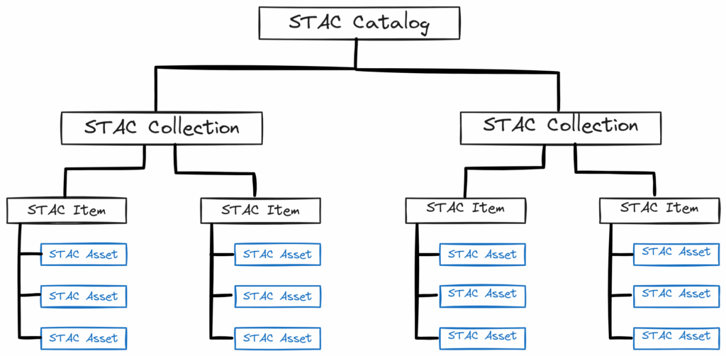
For cloud‑native workflows, STAC is important because:

• It standardises how we describe and organise datasets (including Zarr) so that tools and portals can discover them without custom code for each provider.
• It works equally well as static JSON files in object storage or as dynamic APIs backed by databases, making it flexible for different scales and infrastructures.
• Many ecosystem tools (STAC Browser, PySTAC, STAC API servers, pgSTAC) already understand STAC, so using STAC makes our Zarr data “plug‑and‑play” in that ecosystem.

STAC Catalog

A STAC Catalog is a simple JSON object that links to child Catalogs, Collections, and Items:

JSON

{
  "stac_version": "1.1.0",
  "type": "Catalog",
  "id": "root-catalog",
  "title": "ERA5 Zarr Data Catalog",
  "description": "Root catalog for our cloud-native Zarr data",
  "links": [
    {
      "rel": "child",
      "href": "./era5-zarr/collection.json",
      "type": "application/json"
    },
    /* ... */
  ]
}

The Catalog acts as a top-level entry point for browsing and searching the dataset hierarchy. It can link to other Catalogs, Collections, or Items via links with rel values like child, item, or collection. More details on the Catalog spec.

STAC Collection

A STAC Collection extends Catalog with extra fields describing a coherent group of Items:

JSON

{
  "stac_version": "1.1.0",
  "type": "Collection",
  "id": "era5-zarr",
  "description": "ERA5 surface Zarr datacubes",
  "license": "CC-BY-4.0",
  "extent": {
    "spatial": { "bbox": [[-180, -90, 180, 90]] },
    "temporal": { "interval": [["1950-01-01T00:00:00Z", null]] }
  },
  "keywords": ["reanalysis", "atmosphere", "zarr"],
  "links": [
    {
      "rel": "parent",
      "href": "../catalog.json",
      "type": "application/json",
      "title": "ERA5 Zarr Data Catalog"
    },
    {
      "rel": "item",
      "href": "../items/era5-zarr-2020.json",
      "type": "application/geo+json"
    }
  ]
}

Here, extent describes the spatial and temporal coverage of the collection, license indicates usage rights, and keywords help with discovery. The links section connects to parent Catalogs and child Items. More details and the full list of fields are available on the Collection spec.

STAC Item

A STAC Item is the smallest unit in STAC, an atomic bundle of inseparable metadata and assets. It represents the data at a specific place and time. It is a GeoJSON Feature with additional STAC fields:

JSON

{
  "stac_version": "1.1.0",
  "type": "Feature",
  "id": "era5-zarr-2020",
  "bbox": [
    0,
    -90,
    360,
    90
  ],
  "geometry": { "type": "Polygon", "coordinates": [/* ... */] },
  "properties": {
    "start_datetime": "2020-01-01T00:00:00Z",
    "end_datetime": "2020-12-31T23:59:59Z",
  },
  "collection": "era5-zarr",
  "links": [],
  "assets": {
    "data": {
      "href": "s3://my-bucket/path/to/data.zarr",
      "media_type": "application/vnd+zarr",
    }
  }
}

An Item has a geometry and bbox for spatial coverage, properties for temporal coverage and other metadata, and an assets dictionary that points to the actual data files (e.g. Zarr or Icechunk store in object storage). See the Item spec for more details.

STAC and cloud-native Zarr workflows

---

For Zarr datasets in object storage:

• Each Zarr store is typically referenced as an asset in a STAC Item pointing to the store’s root (e.g. s3://bucket/path.zarr).
• Collections can group multiple Zarr stores that share a product (e.g. “ERA5 surface daily Zarr cubes” or “CMIP6 model X Zarr outputs”).
• Catalogs provide top-level organisation (e.g. per provider, per project).

Benefits for cloud-native workflows:

• STAC makes Zarr datasets “discoverable” by spatial/temporal criteria and keywords, rather than “hidden” as raw paths in buckets.
• Tools like STAC Browser can display and search your STAC catalog or API, making Zarr assets visible in a generic UI.
• STAC API servers backed by databases (e.g. pgSTAC/PgPystac) can support fast, scalable search over many Zarr datasets. More information on STAC API and pgSTAC documentation.

Examples of STAC + Zarr in the wild

STAC is already being used to organise and publish Zarr datasets in operational and research settings. A few good examples are:

• NOC STAC Catalog: The NOC Ocean Data Store publishes oceanographic Zarr datasets as STAC Collections and Items, making them discoverable and accessible via a web interface.
• EOPF Sentinel Explorer: The catalog exposes Sentinel Zarr samples as STAC Collections and Items, and you can inspect individual datasets directly in the browser. This is the link for the STAC API.
• Microsoft Planetary Computer: Searchable spatiotemporal metadata describing Earth science datasets hosted by the Microsoft Planetary Computer. This is the link for the STAC API.

These examples all follow the same idea: STAC describes the dataset, while the Zarr store remains the actual data asset. That makes the data easier to search, browse, and share without inventing a custom metadata format for each project

PySTAC basics: creating Catalogs, Collections, and Items

---

PySTAC is a Python library for working with STAC objects in code, mirroring the JSON structure. You can create Catalogs, Collections, and Items programmatically, add metadata and assets, and save them as JSON files or feed them into a STAC API.

Create a catalog

In this example, we will use the Zarr dataset created in the NetCDF to Zarr conversion lesson. The original data is a subset of the ERA5 reanalysis (data/daily_swh/*.nc) containing the significant wave height (swh) variable. Instead of converting the NetCDF files again, we will use the Zarr dataset that has already been generated and uploaded to the object store.

The first step is to create a root Catalog. A Catalog is the top-level entry point of a STAC hierarchy and can contain one or more Collections.

PYTHON

import pystac

catalog = pystac.Catalog(
    id="Era5-Catalog",
    description="Root catalog for ERA5 datasets"
)

In this example, the Catalog represents all variables available from the ERA5 reanalysis. You can add Collections (or other Catalogs) to it using add_child().

Create a collection

A STAC Collection groups related Items and describes their shared metadata, such as their spatial and temporal extent, license, and description.

Here, we will create a Collection for the significant wave height (swh) dataset. To define its spatial and temporal extent, we first open the Zarr dataset and extract its bounding box and time range.

PYTHON

import xarray as xr

url = "https://atlantis-vis-o.s3-ext.jc.rl.ac.uk/cloud-native-geoscience-course/daily_swh"
ds = xr.open_zarr(url, consolidated=True)
# Get spatial extent (bounding box)
lon_min, lon_max = float(ds.longitude.min()), float(ds.longitude.max())
lat_min, lat_max = float(ds.latitude.min()), float(ds.latitude.max())
# Get temporal extent (start and end time)
time_min, time_max = ds.time.min().values, ds.time.max().values

print(f"Spatial extent: lon [{lon_min}, {lon_max}], lat [{lat_min}, {lat_max}]")
print(f"Temporal extent: time [{time_min}, {time_max}]")

For this tutorial, we will define the Collection as covering the years 2000–2026, even though the example dataset represents only a subset of that period.

PYTHON

from datetime import datetime

extent = pystac.Extent(
    spatial=pystac.SpatialExtent(bboxes=[[lon_min, lat_min, lon_max, lat_max]]),
    temporal=pystac.TemporalExtent(intervals=[[datetime(2000, 1, 1), datetime(2026, 12, 31)]])
)


collection = pystac.Collection(
    id="era5-zarr-swh",
    description="ERA5 surface Zarr datacubes for significant wave height (swh)",
    extent=extent,
    license="CC-BY-4.0"
)

Add the Collection to the Catalog:

PYTHON

catalog.add_child(collection)

Create an item pointing to a Zarr store

An Item represents a single dataset within a Collection. It contains metadata describing the dataset, including its spatial footprint, temporal coverage, and one or more Assets that point to the data itself.

We will create an Item representing the Zarr dataset. Its geometry and bounding box come from the dataset coordinates, while its temporal coverage is taken from the first and last timestamps.

PYTHON

from shapely.geometry import box
import pandas as pd

bbox = [lon_min, lat_min, lon_max, lat_max]
geom = box(*bbox).__geo_interface__

# Convert time to datetime objects
start_datetime = pd.Timestamp(time_min).to_pydatetime()
end_datetime = pd.Timestamp(time_max).to_pydatetime()

item = pystac.Item(
    id="era5-zarr-swh-2025",
    geometry=geom,
    bbox=bbox,
    datetime=None,
    start_datetime=start_datetime,
    end_datetime=end_datetime,
    properties={
        "description": "ERA5 surface Zarr datacube for swh for 2025"
    }
)

Next, create an Asset that points to the Zarr store. The Asset contains the location of the data and describes its format.

PYTHON

url = "https://atlantis-vis-o.s3-ext.jc.rl.ac.uk/cloud-native-geoscience-course/daily_swh"
asset = pystac.Asset(
    href=url,
    media_type="application/vnd+zarr", # Media type for Zarr stores. For icechunk stores, use "application/vnd.zarr+icechunk".
    roles=["data"]
)

Attach the Asset to the Item:

PYTHON

# Add a Zarr asset
item.add_asset("data", asset)

Finally, add the Item to the Collection:

PYTHON

collection.add_item(item)

This completes a minimal STAC hierarchy consisting of a Catalog, which contains a Collection, which in turn contains an Item pointing to a Zarr dataset stored in the object store.

Save as a static catalog (JSON files)

To save the Catalog, Collection, and Item as static JSON files in a directory (e.g. stac/), use the normalize_and_save() method:

PYTHON

catalog.normalize_and_save(
    "stac",
    catalog_type=pystac.CatalogType.SELF_CONTAINED,
)

This will create catalog.json (catalog), era5-zarr-swh/collection.json (collection), and era5-zarr-swh/era5-zarr-swh-2025/era5-zarr-swh-2025.json (item) in the stac/ directory. It will normalize the links so that they are relative to the catalog root, making it easy to upload the entire directory to an object store or web server.

Challenge

Exercise 1 - Build a STAC catalog for your Zarr dataset

Using the Zarr dataset you generated in the NetCDF to Zarr conversion lesson:

1. Create a root Catalog with a clear description.
2. Create a Collection describing your dataset group (e.g. “Example Zarr conversions”).
3. Create an Item whose assets include your Zarr store (Object Store URL).
4. Use catalog.normalize_and_save() to write a static STAC catalog to a stac/ directory.

Questions:

• How did you choose the id, description, and extent for your Collection?
• What information did you include in the Item’s properties and assets to make the Zarr dataset discoverable?

Show me the solution

Create a STAC catalog with a clear description, a Collection with an appropriate extent and license, and an Item that points to the Zarr store. Use PySTAC to save the catalog as JSON files. Include relevant metadata in the Collection and Item to make the dataset discoverable.

STAC in databases: pgSTAC / PgPystac

---

Static STAC catalogs (JSON files in object storage or on a web server) are simple to publish and work well for small to medium datasets.

As the number of Items grows (e.g. millions of scenes or many Zarr datacubes), searching via JSON files becomes less efficient. Many deployments therefore store STAC metadata in a database (like pgSTAC) and expose it via a STAC API. This allows for fast queries, filtering, and pagination. Advantages of database-backed STAC:

• Fast spatial/temporal and attribute queries over large catalogs.
• Indexes and query planners handle complex filters.
• Single source of truth for STAC metadata that can be updated transactionally.

Challenge

Exercise 2 - Discuss JSON vs database-backed STAC

1. When would you prefer a simple static STAC catalog (JSON files in object storage)?
2. When would you prefer a database-backed STAC API (pgSTAC/PgPystac)?
3. How might you evolve from a static JSON catalog to a STAC API over time as your collection of Zarr datasets grows?

Show me the solution

Static STAC is ideal for simple, low-maintenance publishing, while database-backed STAC scales better for large collections and complex search. You might start with a static catalog for a small number of Zarr datasets, and as your collection grows, migrate to a database-backed STAC API to support efficient queries and updates.

Checklist

Visualising your catalog with STAC Browser

STAC Browser is a web application for browsing static STAC catalogs and STAC APIs as a human‑friendly UI.

To visualise your catalog:

1. Upload your stac/ directory to a web server or object storage bucket. To upload the files, you can use boto3 commands in python:

PYTHON

import boto3
from botocore.config import Config
import os

s3 = boto3.client(
    "s3",
    endpoint_url="https://atlantis-vis-o.s3-ext.jc.rl.ac.uk",
    aws_access_key_id="your-access-key",
    aws_secret_access_key="your-secret-key",
    # This is necessary for JASMIN object store, but may not be needed for other S3-compatible stores.
    config=Config(
        request_checksum_calculation="when_required",
        response_checksum_validation="when_required",
    ),
)

bucket_name = "my-bucket" # Replace with your bucket name

for root, dirs, files in os.walk("stac"):
    for file in files:
        local_path = os.path.join(root, file)
        s3_path = os.path.relpath(local_path, "stac")
        s3.upload_file(local_path, bucket_name, f"stac/{s3_path}")

2. With the link to your catalog.json, you can use a hosted STAC Browser demo (e.g. https://browser.moregeo.it/) and enter your catalog URL.

Challenge

Exercise 3 (optional) - Publish and browse your catalog

1. Upload your stac/ directory to the object store.
2. Use a hosted STAC Browser demo.
3. Explore:
   • Your root catalog and collection.
   • The Item representing your Zarr dataset.
   • Asset metadata and links.

Questions:

• How does browsing the STAC catalog compare to looking at raw JSON or Zarr paths?
• What would you add to your STAC metadata to make your Zarr datasets more understandable (keywords, variables, thumbnails, links to documentation)?

Show me the solution

STAC makes their Zarr datasets visible in a generic browser without writing custom UI code. You can see how the hierarchical structure of Catalog → Collection → Item → Assets helps users navigate and understand the datasets.

Key Points

• “STAC standardises how we describe and organise geospatial assets, including Zarr data cubes, making them easier to discover and integrate into cloud-native workflows.”
• “Catalogs, Collections, and Items form a three-layer hierarchy: Catalog as entry point, Collection as grouped datasets, Item as individual spatiotemporal assets with linked data files.”
• “PySTAC provides a Python API to create and manage STAC Catalogs, Collections, and Items, and to save them as static JSON catalogs or feed them into STAC APIs.”
• “Zarr stores in object storage can be referenced as STAC Item assets, connecting cloud-native array data to the broader STAC ecosystem.”
• “STAC metadata can be stored either as static JSON (simple publishing) or in databases like pgSTAC/PgPystac (scalable, queryable STAC APIs), and tools like STAC Browser can visualise both.”

Content from Visualizing Multiscale Zarr and GeoZarr

---

Last updated on 2026-08-11 | Edit this page

Overview

Questions

• “How does chunking affect interactive visualisation of Zarr data in the cloud?”
• “What is a multiscale pyramid, and why does it come from Cloud-Optimized GeoTIFF ideas?”
• “What does GeoZarr add on top of Zarr for geospatial visualisation?”
• “How can we use Topozarr to create multiscale Zarr from our example dataset and explore it in a browser?”

Objectives

• “Explain how geospatial Zarr datasets can be visualised efficiently in the browser and in desktop tools.”
• “Describe why chunking and multiscale pyramids are important for interactive visualisation.”
• “Introduce the GeoZarr conventions for geospatial, multiscale Zarr datasets.”
• “Use Topozarr to build a multiscale Zarr dataset from an existing Zarr store.”
• “Understand how browser clients (e.g. OpenLayers, zarrita, zarr-cesium) can render multiscale GeoZarr without a dedicated tiling server.”

Introduction

---

Zarr can be used for web visualisation as well as scientific analysis. Because the data are stored in chunks, browsers or servers can fetch only the pieces needed for the current map view instead of loading the full dataset.

There are two main patterns. In a server-based workflow, a backend reads the Zarr store and serves tiles or images. In a client-side workflow, the browser reads chunks directly from object storage and renders them with WebGL+GPU or similar tools.

We will see now how to prepare a Zarr dataset for interactive visualisation, and how to explore it in a browser using GeoZarr conventions and simple HTML/JS clients. And we understand why chunking, multiscale pyramids, and GeoZarr metadata are important for performance and user experience.

Chunking matters for visualisation

---

Zarr stores multidimensional arrays as many small chunks. For large geospatial datasets (e.g. global grids, satellite imagery), interactive visualisation often means:

• Looking at relatively small windows (map viewports) at a time.
• Zooming and panning, which changes which subset of data is needed.

Because of that, a good chunking should align with the typical viewports, zoom levels and tiles (e.g. 256×256 or 512×512 pixels) so that the viewer can fetch only the chunks needed for the current view. Another consideration is that the chunks should be small enough for fast transfer (tens or hundreds of kilobytes) but large enough to avoid too many separate HTTP requests.

Inefficient chunking (e.g. huge chunks or misaligned shapes) can lead to the forced loading of much more data than needed for each map view, potentially resulting in sluggish interactions, high bandwidth consumption, and a poor user experience.

For geospatial visualisation, we typically prefer chunking along spatial dimensions (x, y) and possibly band/time, with chunk sizes chosen to balance latency and throughput.

Multiscale pyramids

---

The idea of multiscale pyramids comes from the concept of Cloud-Optimized GeoTIFFs (COGs), which are widely used for imagery. COGs store multiple resolutions of the same data in a single file, allowing clients to request only the resolution needed for the current zoom level, improving performance and reducing bandwidth.

Following the same idea, we can create multiscale pyramids in Zarr. Each level of the pyramid is a downsampled version of the original data, allowing viewers to fetch coarse data for low zoom levels and fine data for high zoom levels. Normally, the pyramid is structured as follows:

• Level 0: full-resolution grid.
• Level 1: downsampled (e.g. 2× coarser) version.
• Level 2: further downsampled, and so on.

As benefits, this allows for efficient visualisation at different zoom levels without overwhelming the client with unnecessary data. For example, a global map view can use a low-resolution overview, while a local zoom can fetch high-resolution tiles only for the area of interest.

GeoZarr’s multiscales convention formalises how to store and describe these pyramids in Zarr.

Source

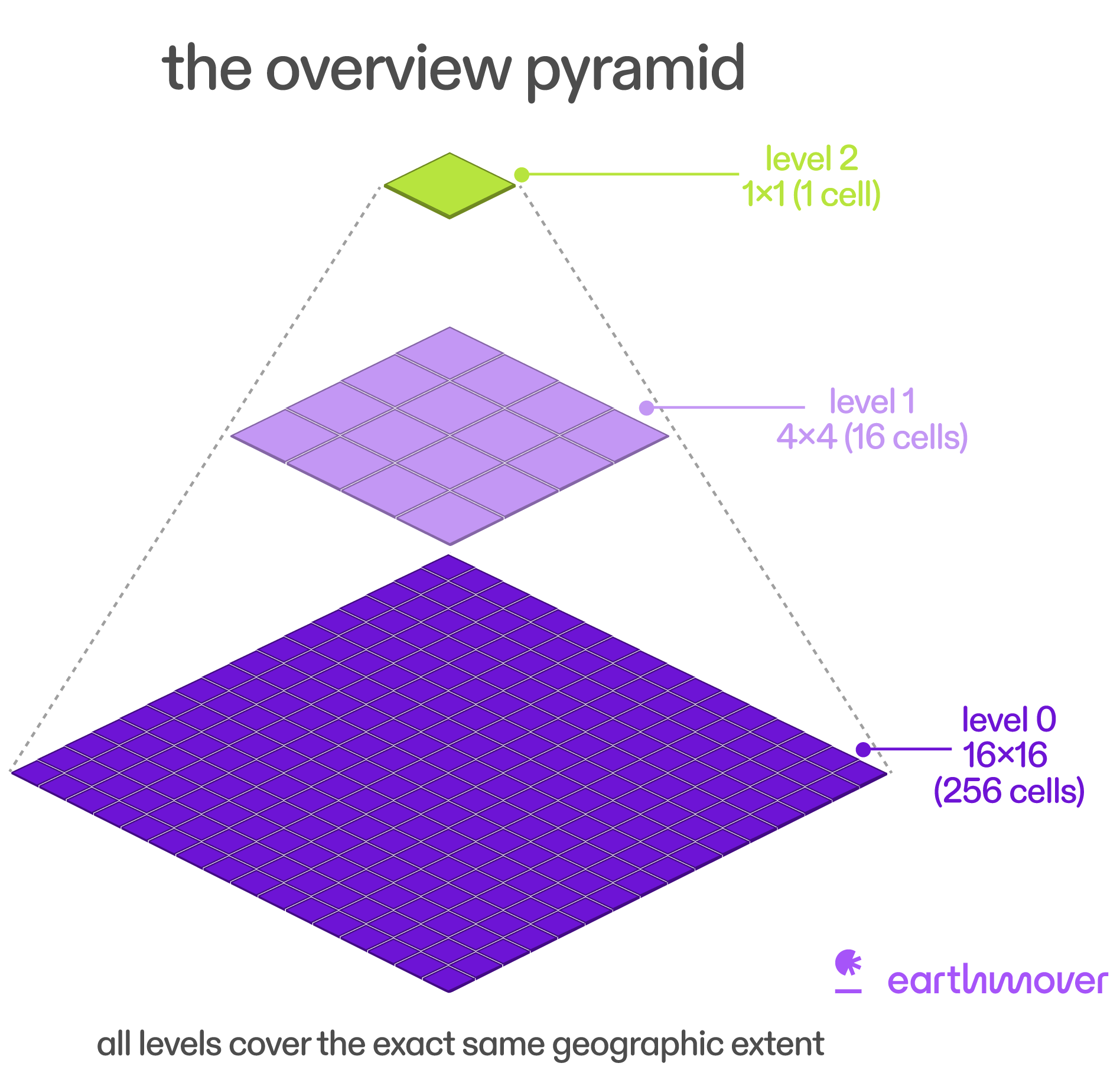
GeoZarr: geospatial conventions for Zarr

---

GeoZarr is a set of modular conventions for encoding geospatial datasets in Zarr. The core conventions include proj, spatial, and multiscales, which describe the coordinate reference system, spatial transforms, and multiscale pyramid structure, respectively.

These conventions are registered via a zarr_conventions metadata attribute and use namespaced attributes like proj:code, spatial:transform, and multiscales. GeoZarr is being developed as an OGC standard that builds upon the Unidata Common Data Model and CF conventions, and aims to bridge scientific and geospatial communities.

Useful references:

• GeoZarr overview: https://geozarr.org
• Conventions (proj, spatial, multiscales): https://geozarr.org/conventions.html
• GeoZarr spec draft: https://zarr.dev/geozarr-spec/documents/standard/template/geozarr-spec.html

Challenge

Exercise 1 - Design a multiscale strategy

Creating a multiscale Zarr store requires some design decisions. Before implementing it, think about your dataset and how you want to visualise it. Because it can be resource-intensive to create multiple levels, we are going to use a small example dataset for this exercise, the data/era5_sst/ocean_temperature.zarr, related to the subset of ERA5 Reanalysis dataset.

1. Look at your example Zarr dataset (dimensions, spatial resolution, domain).
2. Propose:
   • Number of levels (e.g. 3-5).
   • Downsampling method (e.g. mean, min, max, nearest).
   • Spatial chunk size (e.g. 256×256 or 512×512).
3. Discuss with a neighbour:
   • How your choices affect visualisation at different zoom levels.
   • How they might impact performance and storage.

Write down your multiscale plan. You’ll implement it with Topozarr in the next exercise.

Show me the solution

The multiscale strategy will depend on the dataset’s spatial resolution and the desired zoom levels for visualisation. For example, if the original dataset has a resolution of 0.1 degrees, you might choose: - Levels: 4 (0.1°, 0.2°, 0.4°, 0.8°) - Downsampling: mean (to preserve average values) - Chunk size: (256, 256) for spatial dimensions

Topozarr: creating multiscale Zarr for visualisation

---

Topozarr is a Python library from CarbonPlan that helps create multiscale Zarr stores for visualisation, following the GeoZarr conventions. It can take an existing Zarr dataset and generate multiple resolution levels (pyramid) with appropriate metadata.

First, load the zarr dataset using xarray:

PYTHON

import xarray as xr

base_path = "/gws/ssde/j25b/atlantis_vis/cloud-native-geoscience-course/" # or "" if you have the data in your current working directory

ds = xr.open_zarr(f"{base_path}data/era5_sst/ocean_temperature.zarr", consolidated=True)

To generate the multiscale pyramid, you need to set the CRS in the dataset attributes. For example, if the dataset uses WGS84 (EPSG:4326), you can set it like this:

PYTHON

ds = ds.proj.assign_crs({"EPSG": 4326})

PYTHON

from topozarr import create_pyramid

pyramid = create_pyramid(
    ds,
    levels=2, # number of downsampled levels
    x_dim="longitude", # x dimension name
    y_dim="latitude", # y dimension name
    target_chunk_bytes=512 * 512 * 4,  # target chunk size in bytes (e.g. 512x512 pixels with float32)
    method="mean",   # or 'nearest', etc.
    chunks_per_shard=4 # number of chunks per shard for better performance
)

The pyramid is a Pyramid object. In order to take a look at the levels and their shapes, you can convert it to a datatree and inspect the levels:

PYTHON

pyramid_tree = pyramid.as_datatree()
print(pyramid_tree)
print(pyramid_tree["0"])  # Level 0 (full resolution)
print(pyramid_tree["1"])  # Level 1 (downsampled)

Instead of saving each pyramid level as a separate dataset, TopoZarr can write the entire pyramid to a single multiscale Zarr store that follows the GeoZarr conventions. In this example, we will save the multiscale dataset directly to an object store so that it can be accessed efficiently from a web browser:

First, create a mapper for the Zarr store. You can use zarr.storage.FsspecStore to write to an S3 bucket or other object storage:

PYTHON

import xarray as xr
import zarr
import os

store_url = "s3://my-bucket/ocean_temperature_pyramid.zarr"

storage_options = {
    "key": os.environ["AWS_ACCESS_KEY_ID"],
    "secret": os.environ["AWS_SECRET_ACCESS_KEY"],
    "client_kwargs": {"endpoint_url": "https://atlantis-vis-o.s3-ext.jc.rl.ac.uk"},
    "config_kwargs": {
        "request_checksum_calculation": "when_required",
        "response_checksum_validation": "when_required",
    },
}

# Create a reference for the object store
store = zarr.storage.FsspecStore.from_url(
    store_url,
    storage_options=storage_options,
)

Because this task can be resource-intensive, you may want to use a local cluster:

PYTHON

from dask.distributed import Client

client = Client(n_workers=4, threads_per_worker=2, memory_limit="4GB")

And then save the pyramid to the Zarr store:

PYTHON

pyramid_tree.to_zarr(
    store,
    mode="w",
    consolidated=True, # You can set to False for performance
    encoding=pyramid.encoding, # You need to set the encoding as the same encoding in the Pyramid object
    align_chunks=True
)

Now, you can inspect the Zarr hierarchy in the object store to see how the multiscale levels are organised and check for metadata related to multiscales. Because it is a datatree, you need to use the xr.open_datatree function to open the multiscale Zarr store:

PYTHON

import xarray as xr
url = "https://atlantis-vis-o.s3-ext.jc.rl.ac.uk/cloud-native-geoscience-course/ocean_temperature_pyramid.zarr"
ds_pyramid = xr.open_datatree(url, engine="zarr") # remember to use the correct engine for datatree
print(ds_pyramid)

Caution

Watch API churn

Support for multiscale pyramids is a relatively recent addition to the Zarr ecosystem. One of the libraries providing this functionality is Topozarr.

As the Zarr ecosystem continues to evolve, Topozarr is also under active development. As a result, the API for creating multiscale pyramids may change between releases. Always refer to the documentation for the specific version you are using, and consider pinning your package versions to ensure reproducible workflows and avoid unexpected breakages when upgrading dependencies.

Challenge

Exercise 2 - Build and save a multiscale Zarr store

Using the multiscale strategy you designed in Exercise 1, implement it with Topozarr and save the resulting multiscale Zarr store to an object store. Then, inspect the Zarr hierarchy and metadata.

Questions:

• How does the multiscale structure look compared to the original single-resolution dataset?
• How might different levels be used by a viewer when zooming in and out?

Show me the solution

PYTHON

import xarray as xr
import zarr
from topozarr import create_pyramid

base_path = "/gws/ssde/j25b/atlantis_vis/cloud-native-geoscience-course/" # or "" if you have the data in your current working directory

ds = xr.open_zarr(f"{base_path}data/era5_sst/ocean_temperature.zarr", consolidated=True)

ds = ds.proj.assign_crs({"EPSG": 4326})

pyramid = create_pyramid(
    ds,
    levels=2,
    x_dim="longitude",
    y_dim="latitude",
    method="nearest",
    chunks_per_shard=4
)
# Build the multiscale pyramid
pyramid = topozarr.build_pyramid(
    var,
    levels=4,
    downsampling="mean",
    chunk_size=(256, 256)
)

pyramid_tree = pyramid.as_datatree()

# Save the multiscale Zarr store
mapper = "CREATE THE MAPPER"

client = "CREATE A DASK CLIENT"

pyramid_tree.to_zarr(
    store,
    mode="w",
    consolidated=False,
    encoding=pyramid.encoding,
    align_chunks=True
)

Browser-based visualisation: server and client options

---

Once you have a multiscale GeoZarr-compliant Zarr store, you can visualise it in the browser in two main ways: with a server that serves tiles, or with a client that reads Zarr directly from object storage.

Server-side tools read the data on the backend, process it into tiles, and send those tiles to the browser. Client-side tools skip that backend step: they fetch the Zarr chunks directly, choose the right multiscale level, and render in the browser using WebGL.

In both cases, multiscale metadata is important because it tells the viewer which resolution level to use at each zoom level. Good chunking also matters, because viewers work best when the chunks line up reasonably well with the data they need to display.

Server-side visualisation

In the server-side approach, a Python service reads the Zarr data and turns it into map tiles on demand. This is the familiar web-mapping model: the browser asks for tiles, and the server returns ready-to-display images for the current zoom and extent. There are two main options for this:

• TiTiler: dynamic tile services that can render Zarr and other xarray-readable datasets.
• xpublish-tiles: a tile router for xpublish that can serve tiles from xarray/Zarr-backed data.

This approach is useful when you need server-side control over styling, reprojection, access control, or heavy processing. It also works well when you want the browser to stay simple and just consume tiles.

Client-side visualisation

In the client-side approach, the browser reads Zarr chunks directly from object storage and renders them itself. This removes the need for a dedicated tile server, but it means the browser has to do more work.

Examples include:

• zarr-maps: a client-side layer for Leaflet and OpenLayers-style web maps.
• zarr-cesium: client-side visualisation for 2D and 3D in CesiumJS.
• zarr-layer / deck.gl-raster: browser rendering built around Zarr chunk loading and GPU display. For Mapbox and Maplibre.

These tools usually rely on a Zarr JavaScript reader such as Zarrita to fetch chunk data from object storage. The browser then combines that data with WebGL and the GPU to render images, surfaces, or map tiles efficiently.

Source

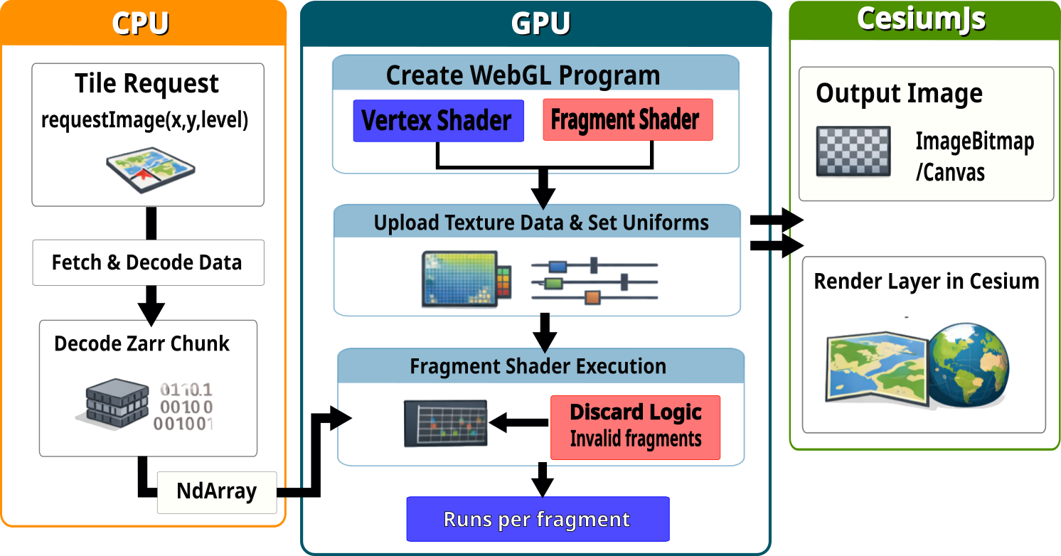
Simple HTML example

In this lesson, we will not go deep into front-end code, but we will show a simple browser example that you can run locally and point at their own multiscale Zarr store. It is the zarr-maps-openlayers.html, which is a minimal HTML page that uses zarr-maps with OpenLayers to visualise a multiscale zarr dataset in the browser.

The lesson renders the same example inline below so you can inspect it directly in the page:

Challenge

Exercise 3 - Explore your multiscale Zarr in the browser

1. In the page above, edit the zarrUrl and variable, add your multiscale zarr dataset.

2. Edit the HTML file zarr-maps-openlayers.html to point to your multiscale Zarr store and the variable you want to visualise.

3. Run a local web server in the directory containing the HTML file:

   BASH

   python -m http.server 8000

   Then open http://localhost:8000/zarr-maps-openlayers.html in your browser.

4. Pan and zoom the map, observing how data loads and renders at different scales.

Questions:

• How responsive is the visualisation, and how does it change as you zoom?
• What might you adjust in your multiscale strategy (levels, chunk size) to improve performance?

Show me the solution

You should experience direct browser-based visualisation of your multiscale Zarr data. You will see how multiscale pyramids and chunking decisions affect the responsiveness and smoothness of interaction.

Challenge

Exercise 4 - Open your multiscale Zarr with zarr-cesium

Open the https://noc-oi.github.io/zarr-cesium/ and enter the URL of your multiscale Zarr store in the input field. You may need to specify additional parameters depending on your dataset (e.g. group name, band selection).

Try to play a little with the controls, zooming and panning around the globe. Observe how the data loads and renders at different zoom levels.

Try to play with one of the Zarr-Cube and Zarr-Cube-Velocity examples, which are designed for 3D visualisation of multiscale Zarr datasets.

Show me the solution

You should experience direct browser-based visualisation of your multiscale Zarr data in 3D. You will see how multiscale pyramids and chunking decisions affect the responsiveness and smoothness of interaction, especially when rotating and zooming around the globe.

The integration of WebGL and GPU acceleration allows for efficient rendering of large datasets without a dedicated tiling server.

Callout

Pipeline for dataset conversion and visualisation

In Lesson 10, we converted a NetCDF dataset into Zarr. In this lesson, we built on that workflow by generating a multiscale Zarr pyramid with TopoZarr and visualising it in a web browser using the GeoZarr conventions.

This extends the original conversion pipeline with an additional multiscale processing step before visualisation.

For datasets on regular grids, the workflow is relatively straightforward. However, many geoscience datasets use irregular or curvilinear grids, where the relationship between Zarr chunks and map tiles is not direct. The NEMO Near-Present-Day dataset is a good example of this. In these cases, it is often necessary to reproject or resample the data onto a regular grid before generating the multiscale pyramid.

Several Python libraries can help with this preprocessing step, including rioxarray, xESMF, and rasterio. For a detailed discussion of the available approaches and their performance, see the Development Seed report: Reprojecting and Resampling Geospatial Data with Python. These tools can help prepare datasets for efficient multiscale visualisation, particularly when working with irregular grids or non-standard map projections.

The diagram below shows the full pipeline, from NetCDF to multiscale Zarr pyramid, ready for browser-based visualisation.

Key Points

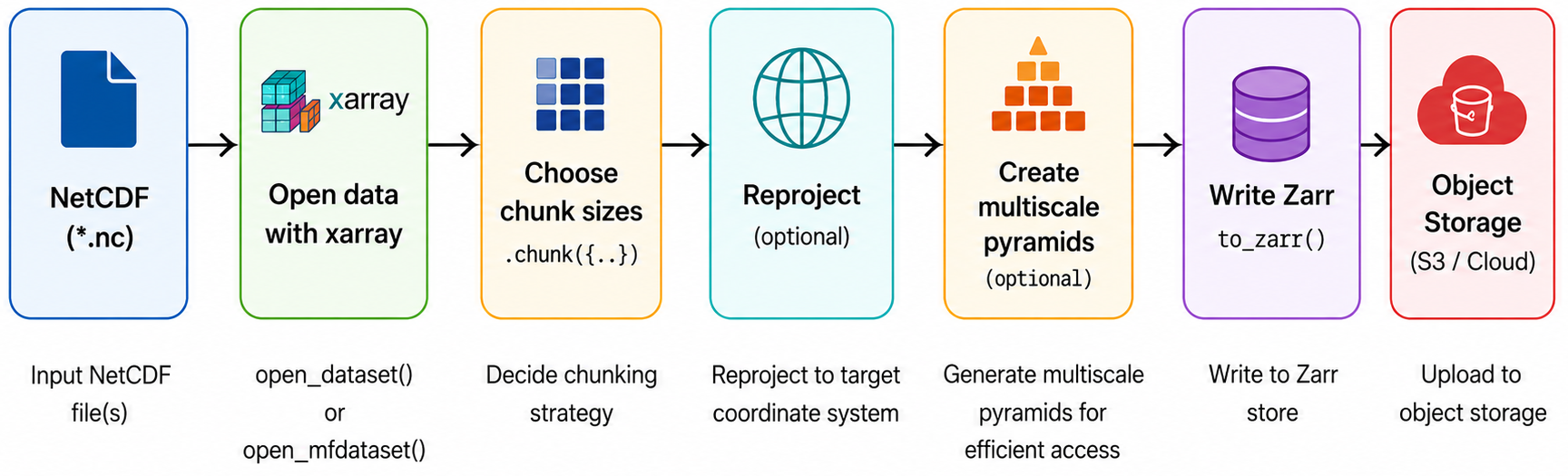
• “Chunking and multiscale pyramids are central to interactive visualisation of geospatial Zarr datasets, allowing efficient tile-based access at different zoom levels.”
• “GeoZarr defines modular conventions (proj, spatial, multiscales) for encoding geospatial metadata and multiscale layouts on top of Zarr.”
• “Topozarr can be used to build multiscale Zarr stores from existing datasets, preparing them for efficient visualisation.”
• “Browser clients such as OpenLayers (GeoZarr source), zarrita, and zarr-cesium can render Zarr data directly from object storage using WebGL and GPU acceleration, without a dedicated tiling server.”
• “By combining GeoZarr conventions, multiscale Zarr, and simple HTML/JS clients, you can build fully cloud-native visualisation workflows for your geospatial datasets.”

Content from Architecture and Best Practices

---

Last updated on 2026-08-05 | Edit this page

Overview

Questions

• “What does a good cloud‑native architecture for geospatial and climate data look like?”
• “How do we decide when to use physical Zarr, virtual Zarr, STAC, Icechunk, GeoZarr, and multiscale pyramids?”
• “What practices help keep data systems robust, reproducible, and future‑proof?”

Objectives

• “Reflect on how the different tools and formats fit together into end‑to‑end architectures.”
• “Identify trade‑offs between simplicity, performance, cost, and maintainability.”
• “Discuss best practices for designing cloud‑native workflows with Zarr, STAC, Icechunk, Virtualizarr, and GeoZarr.”

Why architecture and practice matter

---

Over the course of the lessons, you have seen many building blocks: formats (NetCDF, Zarr), metadata (CF Conventions), object storage, virtualisation (Virtualizarr), versioning (Icechunk), cataloguing (STAC), and visualisation (GeoZarr, multiscale pyramids). Each solves a specific problem, but they only deliver real value when combined into coherent architectures.

A good architecture makes it easy to discover data, access it efficiently, update it safely, and visualise it interactively, while still being understandable and maintainable by your team. Best practices are the habits and patterns that keep such architectures healthy over time: clear metadata, sensible chunking, documented decisions, and automation for repetitive tasks.

Challenge

Exercise 1 - Sketch an end‑to‑end architecture

Individually or in small groups:

1. Sketch an architecture for a hypothetical project (e.g. a global reanalysis, an ensemble forecast system, or a satellite product).
2. Decide:
   • Where raw data lives (formats, storage).
   • How to handle metadata.
   • How and when you convert to Zarr or virtual Zarr.
   • How you apply versioning (Icechunk) and cataloguing (STAC).
   • How users discover, analyse, and visualise data (e.g. GeoZarr, browser tools).
3. Capture your choices and the reasoning behind them in a few bullet points.

Share and discuss:

• Where did you prioritise simplicity?
• Where did you invest in more complex tooling for performance or governance?

Show me the solution

Challenge

Exercise 2 - Draft your personal best‑practice checklist

Take 5-10 minutes to draft a short checklist for future projects, for example:

• “Always define clear metadata and vocabularies for new datasets.”
• “Plan chunking and multiscale layout based on expected access patterns, not just defaults.”
• “Use STAC for discovery and Zarr for analysis. Keep them in sync.”
• “Adopt versioning (Icechunk or similar) for any dataset that is updated regularly.”
• “Prefer virtualisation (Virtualizarr, kerchunk) when full conversion is impractical.”
• “Document architectural decisions and revisit them periodically.”

Compare your checklist with a neighbour’s and refine it into something you might actually use in your own work.

Show me the solution

Key Points

• “Cloud-native workflows are strongest when formats, metadata, storage, and operations are designed together as one architecture.”
• “There is no single best stack: choices between physical Zarr, virtual Zarr, STAC, Icechunk, and GeoZarr depend on workload, governance, and resources.”
• “Practical trade-offs among simplicity, performance, cost, and maintainability should be documented and revisited over time.”
• “Chunking, metadata quality, and discoverability are foundational decisions that strongly affect usability and long-term sustainability.”
• “A short, explicit best-practice checklist helps teams apply course concepts consistently in real projects.”