Image 1 of 1: ‘'data' is a 3 by 3 numpy array containing row 0: ['A', 'B', 'C'], row 1: ['D', 'E', 'F'], and row 2: ['G', 'H', 'I']. Starting in the upper left hand corner, data[0, 0] = 'A', data[0, 1] = 'B', data[0, 2] = 'C', data[1, 0] = 'D', data[1, 1] = 'E', data[1, 2] = 'F', data[2, 0] = 'G', data[2, 1] = 'H', and data[2, 2] = 'I', in the bottom right hand corner.’
Figure 2
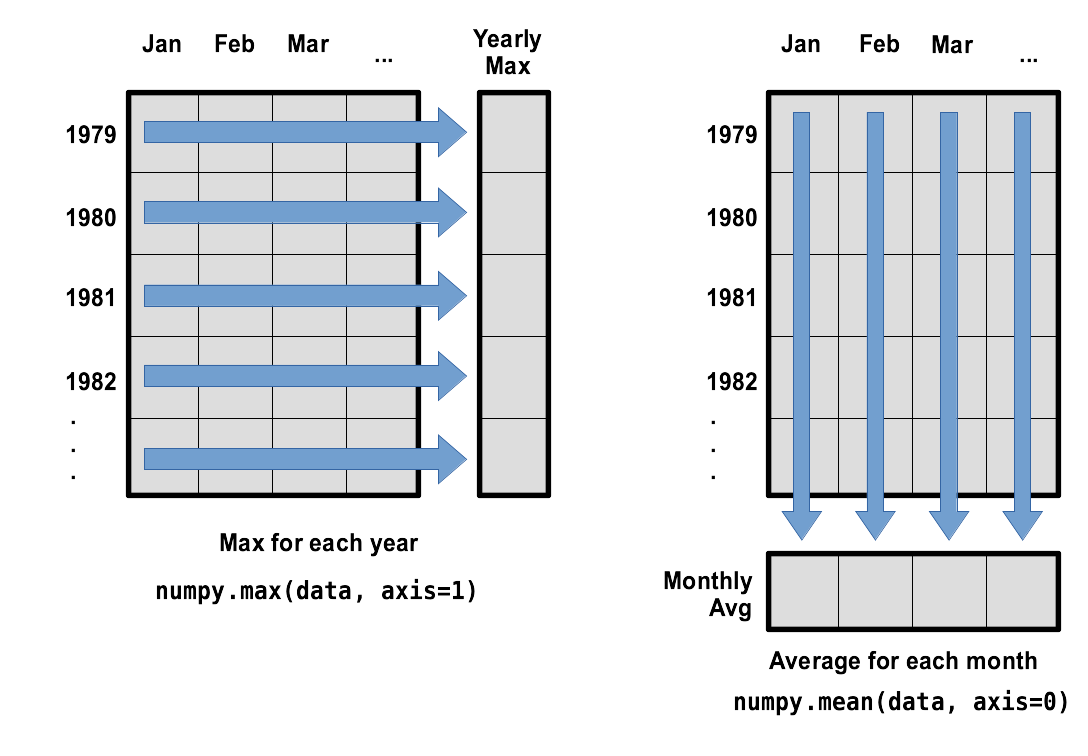
Image 1 of 1: ‘Per-year maximum height is computed row-wise across all columns using numpy.max(data, axis=1). Per-year average wave height is computed column-wise across all rows using numpy.mean(data, axis=0).’
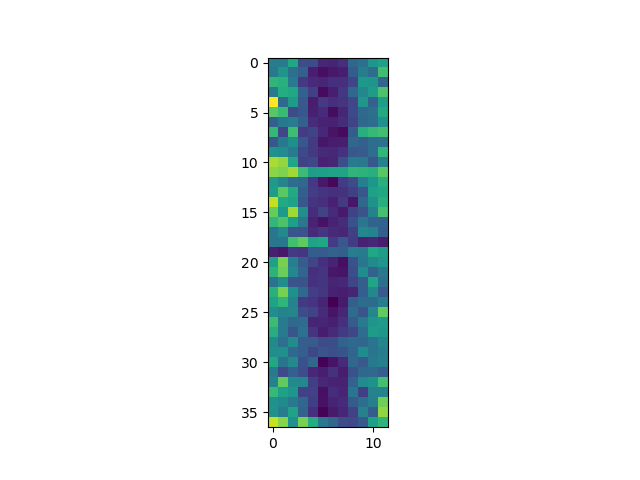
Image 1 of 1: ‘Heat map representing the wave height from the first 50 days. Each cell is colored by value along a color gradient from blue to yellow.’
Figure 2
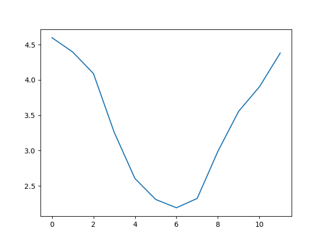
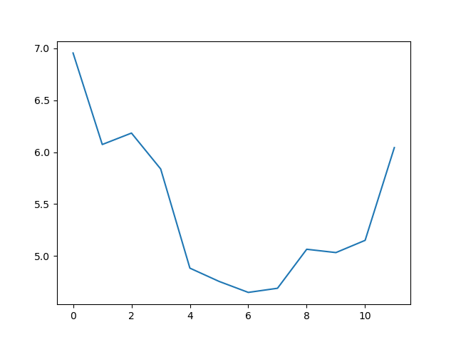
Image 1 of 1: ‘A line graph showing the monthly average wave height over a 37 year period.’
Figure 3
Image 1 of 1: ‘A line graph showing the maximum wave height per month over a 37 year period.’
Figure 4
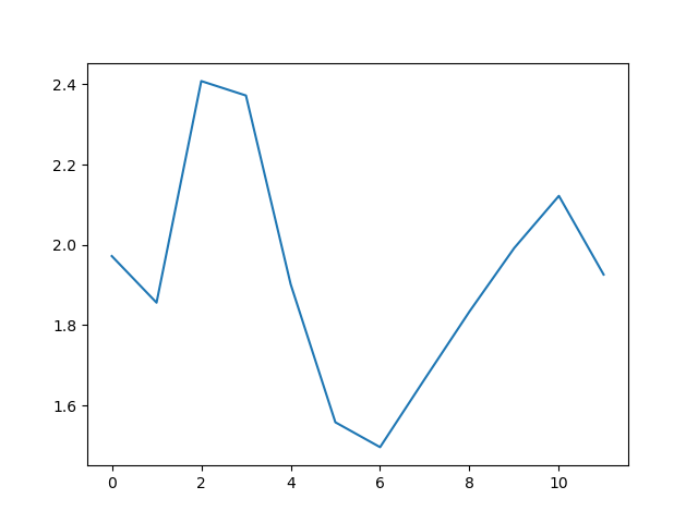
Image 1 of 1: ‘A line graph showing the minimum wave height per month over a 37 year period.’
Figure 5
Image 1 of 1: ‘Three line graphs showing the daily average, maximum and minimum wave-heights over a 446-day period.’
Figure 6
Image 1 of 1: ‘Three plots showing the average, maximum and minimum waveheights plotted on a single pair of axes.’
Figure 7
Image 1 of 1: ‘Global surface waveheight’
Figure 8
Image 1 of 1: ‘Global surface waveheight with a colourbar’
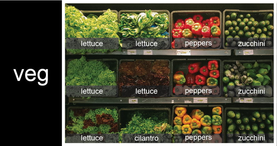
Image 1 of 1: ‘veg is represented as a shelf full of produce. There are three rows of vegetables on the shelf, and each row contains three baskets of vegetables. We can label each basket according to the type of vegetable it contains, so the top row contains (from left to right) lettuce, lettuce, and peppers.’
Figure 2
Image 1 of 1: ‘veg is now shown as a list of three rows, with veg[0] representing the top row of three baskets, veg[1] representing the second row, and veg[2] representing the bottom row.’
Figure 3
Image 1 of 1: ‘veg is now shown as a two-dimensional grid, with each basket labeled according to its index in the nested list. The first index is the row number and the second index is the basket number, so veg[1][3] represents the basket on the far right side of the second row (basket 4 on row 2): zucchini’
To reference a specific basket on a specific shelf, you use two
indexes. The first index represents the row (from top to bottom) and the
second index represents the specific basket (from left to right).


!['data' is a 3 by 3 numpy array containing row 0: ['A', 'B', 'C'], row 1: ['D', 'E', 'F'], and row 2: ['G', 'H', 'I']. Starting in the upper left hand corner, data[0, 0] = 'A', data[0, 1] = 'B', data[0, 2] = 'C', data[1, 0] = 'D', data[1, 1] = 'E', data[1, 2] = 'F', data[2, 0] = 'G', data[2, 1] = 'H', and data[2, 2] = 'I', in the bottom right hand corner.](../fig/python-zero-index.svg)


![veg is now shown as a list of three rows, with veg[0] representing the top row of three baskets, veg[1] representing the second row, and veg[2] representing the bottom row.](../fig/04_groceries_veg0.png)
![veg is now shown as a two-dimensional grid, with each basket labeled according to its index in the nested list. The first index is the row number and the second index is the basket number, so veg[1][3] represents the basket on the far right side of the second row (basket 4 on row 2): zucchini](../fig/04_groceries_veg00.png)