Introduction
Overview
Teaching: 20 min
Exercises: 15 minQuestions
What are some of the common computing terms that I might encounter?
How can I use Python to work with large datasets?
How do I connect to a high performance computing system to run my code?
Objectives
To understand common computing terms around using HPC and Jupyter systems.
To understand what JASMIN is and the services it provides.
To have the lesson conda environment installed and running.
To be able to launch a JupyterLab instance with the lesson’s data and code present.
To be aware of the key libraries used in this lesson (Xarray, Numba, Dask, Intake).
How do we scale Python to work with big data?
Python is an increasingly popular choice for working with big data. In enviromental sciences we often encounter data that is bigger than our computer’s memory and/or that is too big to process with our desktop or laptop computers.
What are your needs?
- In the etherpad write a sentence about what kind of data you work with and how big that data is.
- Describe the problems you have working with data that is too big for your desktop or laptop computer to handle.
- List any tools, libraries and computing systems you use or have used to overcome this.
The tools we’ll look at in this lesson
In this lesson we will look at a few tools to help you work with big data and to process your data more efficiently and by using parallel processing, these will include:
- GNU Parallel
- Numpy
- Numba
- Xarray
- Dask
- Zarr
- Intake
Jargon Busting
CPU
At the heart of every computer is the CPU or Central Processing Unit. This takes the form of a microchip and typically the CPU is the biggest microchip in the computer. The CPU can be thought of as the “brain” of the computer and is what ultimately runs all of our software and carries out any operations we perform on our data.
Core
Until around 2010 most CPUs had a single processing core and could only do one thing at a time. They gave the illusion of doing multiple things at once by rapidly switching from one task to another. A few higher end computers would have multiple CPUs and could do 2/4/8 things at once if they had 2/4/8 CPUs. Since around 2010 most CPUs have multiple cores, which is effectively putting multiple CPUs onto a single chip. By having multiple cores modern computers can perform multiple tasks simultaneously.
Node/Cluster
A single computer in a group of computers known as a cluster is often called a “node”. A cluster allows us to run large programs over multiple computers with data being exchanged over a high speed network called an interconnect.
Process
A process is a single running copy of a computer program. If for example launch a (simple) Python program then it will create one Python process to run this. We can see a list of
processes running on a Linux computer with the ps or top command or on windows using the Task Manager. The computer’s operating system will decide which core should run which process
and will rapidly switch between all the running processes to ensure that they all have a chance to do some work. If a process is waiting on input from the user or for data to arrive
from a hardware device such as a disk or network then it might give up its turn to do any work until the input/data arrives. The operating system isolates each process from the others,
each will have its own memory allocated and won’t be able to read or write data to another process’s memory.
Thread
A thread is a way of having multiple things happening simultaneously inside one process. Unlike processes, threads can access each other’s memory. In multicore systems each thread might run on a different core. Some CPUs also have a feature called Hyper Threading where for every core they have some additional parts of a core, this can help run some multithreaded applications a little bit faster while only requiring a small amount of extra ciricuitry in the CPU. Some programs which tell us about the specifications of a CPU will mention how many threads a CPU has, in Hyper Threaded systems this will be double the number of cores, in non-Hyper Threaded systems it will be the same as the number of cores.
Parallel Processing
Parallel Processing is where a task is split across multiple processing cores to run different parts of it simultaneously and make it go faster. This can be acheived by using multiple processes and/or multiple threads. Bigger and more complex tasks might also be split across several computers.
Computer memory
There are two main types of computer memory, RAM or volatile storage and disk or non-volatile storage.
RAM
RAM or Random Access Memory is the computer’s short term memory, any program which is running must be loaded into RAM as is any data which that program needs. When the computer is switched off the contents of the RAM are lost. RAM is very fast to access and the “Random” in the name means it be both read from and written to. A typical modern computer might have a few gigabytes (a few billion characters) worth of RAM.
Storage
Disk or storage or non-volatile storage is where computers store things for longer term keeping. Traditionally this was on a hard disk that had spinning platters which could be magnetised (or before that on removable floppy disks which also magnetise a spinning disk). Many modern computers use Solid State Disks (SSDs) which are faster and smaller than hard disks, but they are still slower than RAM and are often more expensive. A typical modern computer might have a few hundred gigabytes to a few terabytes (trillion characters) worth of disk.
HPC systems will often have very large arrays of many disks attached to them with hundreds of terabytes or even petabytes (1000 TB) between them. On some systems this will include a mix of slower hard disks and faster but less plentiful SSDs. Some systems also have tape storage which can hold large amounts of data but is very slow to access and is typically used for backup or archiving.
Server
A server is a computer connected to a network (possibly including the internet) that accepts connections from client computers and provides them access to some kind of service, sends them some data or receives some data from them. Typically server computers have a large number of CPU cores, disk storage and/or RAM.
High Performance Computing
High Performance Computing (sometimes called Super Computing) refers to large computing systems and clusters that are typically made up of many individual computers with a large number of cores between them. They’re often used for research problems such as processing large environmental datasets or running large models and simulations such as climate models. High Performance Computing (HPC) systems are usually shared between many users. To ensure that one user doesn’t take all the resources for themselves or prevent another users program from running users are required to write a job description which tells the HPC what program they want to run and what resources it will need. This is then placed in a queue and will be run when the required resources are available. Typically when a job runs it will have a set of CPU cores dedicated to it and no other programs (apart from the operating system) will be able to use those cores.

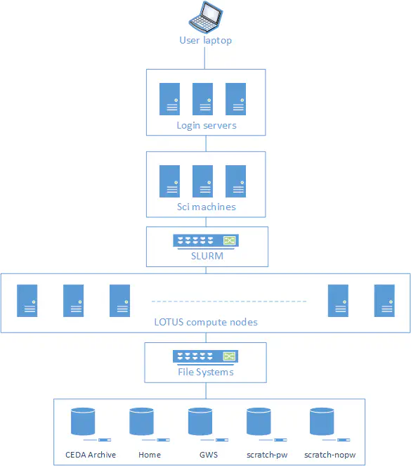
JASMIN
https://jasmin.ac.uk is the UK’s data analysis facility for data intensive environmental science. It combines several computing services together including:
- High Performance Computing system called Lotus with over 19,000 processing cores and 300 nodes.
- Virtual machines
- Jupyter Notebooks service
- Data Storage on both disk and tape
- Moderate sized shared “sci” servers, with between 8 and 48 CPU cores and 32G to 1TB of RAM
SSH
SSH or Secure SHell is a program for connecting to and running commands on another computer over a local network or the internet. As the “secure” part of the name implies, SSH encrypts all the data that it sends so that anybody intercepting the data won’t be able to read it. SSH is used to support accessing the command line interface of another computer, but it can also “tunnel” other data through the SSH connection and this can include the output of graphical programs, allowing us to run graphical programs on a remote computer.
SSH has two accompanying utilities for copying files, called SCP (Secure Copy) and SFTP (Secure File Transfer Protocol) that allow us to use SSH to copy files to or from a remote computer.
Jupyter Notebooks
Jupyter Notebooks are an interactive way to run Python (and Julia or R) in the web browser. Jupyter Lab is the program which runs a Jupyter server that we can connect to. We can run Jupyter Lab on our own computer by downloading Anaconda and running Jupyter Lab via the Anaconda Navigator, when run in this way any Python code written in the Notebook will run on our own computer. We can also use a service called a Jupyter Hub run by somebody else, usually on a server computer. When run in this way any code written in the Notebook will run on the server. This means we can take advantage of the server having more memory, CPU cores, storage or large datasets that aren’t on our computer.
Jupyter Lab also allows us to open a terminal and type in commands that run either on our computer or the Jupyter server. This can be helpful alternative to using SSH to connect to a remote server as it requires no SSH client software to be installed.
Connecting to a JupyterLab/notebooks service
We will be using the Notebooks service on the JASMIN system for this workshop. This will open a Jupyter notebook in your web browser, from this you can type in Python code and it will run on the JASMIN system. JASMIN is the UK’s data analysis facility for environmental science and co-locates both data storage and data processing facilities. It will also be possible to run much of the code in this workshop on your own computer, but some of the larger examples will probably exceed the memory and processing power of your computer.
Launching JupyterLab
In your browser connect to https://notebooks.jasmin.ac.uk. If you have an existing JASMIN account then login with your normal username and password. There is a two factor authentication on the notebook service that will email you a code, enter this code and you will be connected to the Notebook service. If you do not have a JASMIN account then please use one of the training accounts provided.
Download examples and set up the Mamba environment
To ensure we have all the packages needed for this workshop we’ll need to create a new mamba environment (mamba is a conda compatible package manger but is much faster than conda). This is defined by a YAML file that is downloaded alongside the course materials.
Download the course material
Open a terminal and type:
curl https://raw.githubusercontent.com/NOC-OI/python-advanced-esces/gh-pages/data/data.tgz > data.tgz
tar xvf data.tgz
Setting up/choosing a Mamba environment
From the terminal run the following:
curl https://raw.githubusercontent.com/NOC-OI/python-advanced-esces/refs/heads/gh-pages/data/esces-env.yml > esces-env.yml
mamba env create -f esces-env.yml -p ~/.conda/envs/esces
mamba run -p ~/.conda/envs/esces python -m ipykernel install --user --name ESCES
After about one minute if you click on the blue plus icon near the top left or the file menu and “New Launcher” option you should see a notebook option called ESCES. This will use the Mamba environment we just created and will have access to all the packages we need.
Testing package installations
Testing your package installs
Run the following code to check that you can import all the packages we’ll be using and that they are the correct versions. The !parallel runs the parallel command from the command line from within a Jupyter notebook cell. This will not work if you use stanard Python.
import xarray
import dask
import numba
import numpy
import cartopy
import intake
import zarr
import netCDF4
print("Xarray version:", xarray.__version__)
print("Dask version:", dask.__version__)
print("Numpy version:", numpy.__version__)
print("Numba version:", numba.__version__)
print("Cartopy version:", cartopy.__version__)
print("Intake version:", intake.__version__)
print("Zarr version:", zarr.__version__)
print("netCDF4 version:", netCDF4.__version__)
!parallel --version
Solution
You should see version numbers that are equal or greater than the following:
Xarray version: 2024.2.0
Dask version: 2024.3.1
Numpy version: 1.26.4
Numba version: 0.59.0
Cartopy version: 0.22.0
Intake version: 2.0.4
Zarr version: 2.17.1
netCDF4 version: 1.6.5
GNU parallel 20230522
Copyright (C) 2007-2023 Ole Tange, http://ole.tange.dk and Free Software
Foundation, Inc.
License GPLv3+: GNU GPL version 3 or later <https://gnu.org/licenses/gpl.html>
This is free software: you are free to change and redistribute it.
GNU parallel comes with no warranty.

Web site: https://www.gnu.org/software/parallel

When using programs that use GNU Parallel to process data for publication
please cite as described in 'parallel --citation'.
About the example data
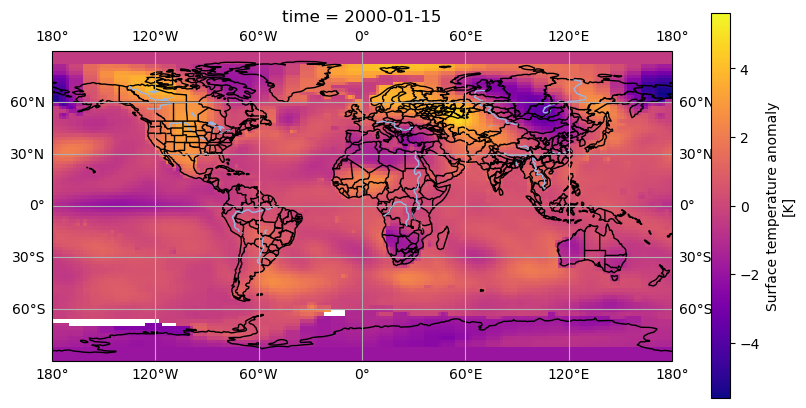
There is a small example dataset included in the download above. This is a Surface Temperature Analysis from the Goddard Institute for Space Studies at NASA. It contains a monthly surface temperatures on a 2x2 degree grid from across the earth from 1880 to 2023. The data is stored in a NetCDF file. We will be using a subset of the data that runs from 2000 to 2023.
About NetCDF files
NetCDF files are suited for storing array data
They are:
- Self Describing, there is a metadata describing the whole dataset, the variables within it and their units.
- Widely supported, there are libraries to read netCDF in most programming languages and lots of tools to manipulate them.
- Python has a NetCDF4 library that can work with them, the Xarray library also works with NetCDF.
- Efficient, can store data in binary formats instead of ASCII data as CSV would.
- Able to contain multiple variables
- Contains three types of data:
- Variables: the actual data.
- Dimensions: the dimensions on which the variables exist, for example latitude, longitude and time.
- Attributes: Information about the dataset, for example who created it and when.
Exploring the GISS Temp Dataset
Load and get an overview of the dataset
import netCDF4
dataset = netCDF4.Dataset("gistemp1200-21c.nc")
print(dataset)
<class 'netCDF4.Dataset'>
root group (NETCDF4 data model, file format HDF5):
    title: GISTEMP Surface Temperature Analysis
    institution: NASA Goddard Institute for Space Studies
    source: http://data.giss.nasa.gov/gistemp/
    Conventions: CF-1.6
    history: Created 2024-03-08 11:37:27 by SBBX_to_nc 2.0 - ILAND=1200, IOCEAN=NCDC/ER5, Base: 1951-1980
    dimensions(sizes): lat(90), lon(180), time(288), nv(2)
    variables(dimensions): float32 lat(lat), float32 lon(lon), int32 time(time), int32 time_bnds(time, nv), int16 tempanomaly(time, lat, lon)
    groups:
Get the list of attributes
dataset.ncattrs()
['title', 'institution', 'source', 'Conventions', 'history']
print(dataset.title)
'GISTEMP Surface Temperature Analysis'
Get the list of variables
print(dataset.variables)
Get the list of dimensions
print(dataset.dimensions)
Read some data from out dataset
The dataset values can be read from dataset.variables['variablename'], it will have a subarray that contains the data following the dimensions specified.
In our dataset we can see that the tempanomaly variable has the shape int16 tempanomaly(time, lat, lon).
This means that time will be the first index, latitude the second and longitude the third. We can get the first timestep for the upper left coordinate by using:
print(dataset.variables['tempanomaly'][0,0,0])
One thing to note here is that our dataset’s y coordinates are backwards to most maps (following a computer graphics convention where 0 is the upper left coordinate, not the lower left or centre).
Therefore requesting [0,0,0] means the southern most and western most coordinate at the first timestep.
Read some NetCDF data
Challenge
There are 90 elements to the latitude dimension, one every two degrees and 180 in the longitude dimension, also with one every two degrees. To translate from a real latitude and longitude to an index we’ll need to divide the longitude by two and add 90 to the longitude. For the latitude we’ll need to divide by two and add 45. In Python this can be expressed as the following, we’ll also want to ensure the result is an integer by wrapping the whole calculation in
int():latitude_index = int(((latitude) / 2) + 45) longitude_index = int((longitude / 2) + 90)For the time dimension, each element represents one month starting from January 2000, so for example element 12 will be January 2001 (0-11 are January to December 2000). For example 52 degrees north (latitude) and 2 degrees west will translate to the array index 71, 91. Write some code to get the temperature anomaly for January 2020 in Astana, Kazakhstan (approximately 51 North, 71 East)
Solution
latitude = 71
longitude = 51
latitude_index = int(((latitude) / 2) + 45)
longitude_index = int((longitude / 2) + 90)
time_index = 20 * 12   #we want jan 2020, dataset starts at jan 2000 and has monthly entries
print(dataset.variables['tempanomaly'][time_index,latitude_index,longitude_index])
6.8999996
Key Points
Jupyter Lab is a system for interactive notebooks that can run Python code, these can be either on own computer or a remote computer.
Python can scale to using large datasets with the Xarray library.
Python can parallelise computation with Dask or Numba.
NetCDF format is useful for large data structures as it is self-documenting and handles multiple dimensions.
Zarr format is useful for cloud storage as it chunks data so we don’t need to transfer the whole file.
Intake catalogues make dealing with multifile datasets easier.
Coffee Break
Overview
Teaching: min
Exercises: minQuestions
Objectives
Feedback
In the etherpad, answer the following questions:
- Are we going too fast, too slow or just write? Record your answer in the etherpad
- What don’t you understand or would like clarification on?
Take a break!
- Drink something
- Eat something
- Talk to each other
- Get some fresh air
Key Points
Dataset Parallelism
Overview
Teaching: 15 min
Exercises: 10 minQuestions
How do we apply the same command to every file or parameter in a dataset?
Objectives
Use GNU Parallel to apply the same command to every file or parameter in a dataset
Dataset Parallelism with GNU Parallel
GNU Parallel is a very powerful command that lets us execute any command in parallel. To do this effectively we need what is often called an “embarrasingly parallel” problem. These are problems where a dataset can be split into several parts and each can be processed independently and simultaneously. Such problems often occur when a dataset is split across multiple files or there are multiple parameters to process.
Basic use of GNU Parallel
In the Unix shell we could loop over a dataset one item at a time by using a for loop and the ls command together.
for file in $(ls) ; do
    echo $file
done
We can ask GNU parallel to perform the same task and at least several of the echo commands will run simultaneously.
The {1} after the echo will be substituted by what ever comes after :::, in this case the output of the ls command.
parallel echo {1} ::: $(ls)
We could also use a set of values instead of ls:
parallel echo {1} ::: 1 2 3 4 5 6 7 8
Just running echo commands isn’t very useful, but we could use parallel to invoke a Python script too. The serial example to process a series of NetCDF files would be:
for file in $(ls *.nc) ; do
    python myscript.py $file
done
And with parllel it would be:
parallel python myscript.py {1} ::: $(ls *.nc)
Citing Software
It is good practice to cite the software we use in research. GNU Parallel is particularly vocal about this and it will remind you to cite it.
Running parallel --citation will show us all of the information we’ll need if we are going to cite it in a publication, it will also prevent further reminders about it.
Working with multiple arguments
The {1} can be used multiple times if we want the same argument to be repeated.
If for example the script required an input and output file name and the output was the input file with .out on the end, then we could do the following:
parallel python myscript-2.py {1} {1}.out ::: $(ls *.nc)
Using a list of files stored in a file
Using commands or lists of arguments is fine for many use cases, but sometimes there are cases where we might want to use a list of files in a text file.
For this we use the :::: (note four, not three :s) separator and specify the file name after that, each line in file will be used as a line of input.
ls *.nc | grep "^ABC" > files.txt
parallel python myscript-2.py {1} {1}.out :::: files.txt
More complex arguments
Parallel can also run two (or more) sets of arguments, the first argument will become {1}, the second {2} and so on. Each argument’s input list must be separated by a :::.
parallel echo "hello {1} {2}" ::: 1 2 3 ::: a b c
We can also mix the ::: and :::: notations to have some arguments come from files and others from lists.
For example, if we had a list of netcdf files in files.txt, and you wanted to perform an analysis of two of the varibles, we could use:
parallel process.py --variable={1} {2} ::: temp sal :::: files.txt
{1} will be substituted for temp or sal, while {2} will be given the filenames. Parallel will run process.py for both variables on every file.
Pairing arguments
Sometimes we don’t want to run every variable with every other variable, but will want to run them in pairs, for example:
parallel echo "hello {1} {2}" ::: 1 2 3 :::+ a b c
which produces:
hello world 1 a
hello world 2 b
hello world 3 c
Job Control
By default Parallel will use every processing core on the system. Sometimes, especially on shared systems this isn’t what we want to do.
On some HPC systems we might only be allocated a few cores, but the system will have many more and Parallel will try to use them all.
Depending on how the system is configured that will either cause us to run several processes on each core we’re allocated or to exceed our allocation.
We can tell Parallel to limit how many cores it is running on with the --max-procs argument.
Logging
In more complex jobs it can be useful to have a log of which jobs ran, when they started and how long they took.
This is set with the --joblog option to Parallel and is followed by a file name. For example:
parallel --joblog=jobs.log echo {1} ::: 1 2 3 4 5 6 7 8 9 10
After Parallel has finished we can look at the contents of the file jobs.log and see the output:
Seq     Host    Starttime       JobRuntime      Send    Receive Exitval Signal  Command
1       :       1711502183.024       0.002      0       2       0       0       echo 1
2       :       1711502183.025       0.003      0       2       0       0       echo 2
3       :       1711502183.026       0.003      0       2       0       0       echo 3
4       :       1711502183.028       0.002      0       2       0       0       echo 4
5       :       1711502183.029       0.003      0       2       0       0       echo 5
6       :       1711502183.030       0.003      0       2       0       0       echo 6
7       :       1711502183.032       0.003      0       2       0       0       echo 7
8       :       1711502183.034       0.004      0       2       0       0       echo 8
9       :       1711502183.036       0.002      0       2       0       0       echo 9
10      :       1711502183.037       0.003      0       3       0       0       echo 10
Timing the speed up with Parallel
There is a script included with the example dataset called plot_tempanomaly.py. This script will plot a map of the temperature anomaly data from our GISS dataset. It takes three arguments, the name of the NetCDF file to use, a start year (specified with –start) and an end year (specified with –end). It will create a PNG file for each month that it processes.
For example to run this for the year 2000 we would run:
python plot_tempanomaly.py gistemp1200-21c.nc --start 2000 --end 2001We can time how long a command takes by prefixing it with the
timecommand, this will return three numbers:
- real: how long the whole command took to run
- user: how much time the command used the processor for in user mode, this is typically within our code and the libraries it calls.
- sys: how much time the command used the processor for in system mode, this typically means the time spent waiting for hardware devices to respond, for example the disk, screen or network. The sys and user time can exceed the real time when multiple processor cores are used.
Run this for the years 2000 to 2023 as a serial job with the commands:
time for year in $(seq 2000 2023) ; do python plot_tempanomaly.py gistemp1200-21c.nc --start $year --end $[$year+1] ; doneNow repeat the command using Parallel:
time parallel python plot_tempanomaly.py gistemp1200-21c.nc --start {1} --end {2} ::: $(seq 2000 2023) :::+ $(seq 2001 2024)Note that if you are using parallel from outside of Jupyter lab then you running parallel decativates your conda/mamba environment. The easiest solution to this is to create a wrapper shell script that runs the python command. Type the following into your favourite text editor and save it as
plot_tempanomaly.sh.#!/bin/bash python plot_tempanomaly.py $1 --start $2 --end $3time parallel bash plot_tempanomaly.sh gistemp1200-21c.nc {1} {2} ::: $(seq 2000 2023) :::+ $(seq 2001 2024)Compare the runtimes of the parallel and serial versions. Try adding the joblog option and examining how many jobs launched at once. How many jobs did Parallel launch simultaneously? How much faster was the parallel version than the serial version? Try adding the –max-procs option and setting this to 2,4 or 8 and compare the run time.
Bonus Challenge: Make a Movie
We now have 288 PNG images covering the time period of our dataset. A useful way to view these would be as a video. There are a number of programs you can use to convert these into a video file. One such program is FFmpeg. You might need to install FFmpeg via Conda/Mamba. Lookup in the FFmpeg documentation how to make your images into a video. Create the video, download it to your computer (you can’t play it in Jupyter Lab) and play it.
Solution
ffmpeg -framerate 25 -pattern_type glob -i "*.png" -c:v libx264 output.mp4
Key Points
GNU Parallel can apply the same command to every file in a dataset
GNU Parallel works on the command line and doesn’t require Python, but it can run multiple copies of a Python script
It is often the simplest way to apply parallelism
It requires a problem that works independently across a set of files or a range of parameters
Without invoking a more complex job scheduler, GNU Parallel only works on a single computer
By default GNU Parallel will use every CPU core available to it
Lunch Break
Overview
Teaching: min
Exercises: minQuestions
Objectives
Feedback
In the etherpad answer the following questions:
- Are we going too fast, too slow or just write? Record your answer in the etherpad
- What’s the most useful thing we’ve covered so far?
- What don’t you understand or would like clarification on?
Have some lunch
- Take a break
- Eat something
- Drink something
- Talk to each other
- Get some fresh air
Key Points
Parallelisation with Numpy and Numba
Overview
Teaching: 50 min
Exercises: 30 minQuestions
How can we measure the performance of our code?
How can we improve performance by using Numpy array operations instead of loops?
How can we improve performance by using Numba?
Objectives
Apply profiling to measure the performance of code.
Understand the benefits of using Numpy array operations instead of loops.
Remember that single instruction, multiple data instrcutions can speed up certain operations that have been optimised for their use.
Understand that Numba is using Just-in-time compilation and vectorisation extensions.
Understand when to use ufuncs to write functions that are compatible with Numba.
This episode is based in material from Ed Bennett’s Performant Numpy lesson
Measuring Code Performance
There are several ways to measure the performance of your code.
Timeit
We can get a reasonable picture of the performance of individual functions and code snippets
by using the timeit module. timeit will run the code multiple times and take an average runtime.
In Jupyter, timeit is provided by line and cell magics. A magic is some special extra helper features added to Python.
The line magic:
%timeit result = some_function(argument1, argument2)
will report the time taken to perform the operation on the same line
as the %timeit magic. Meanwhile, the cell magic
%%timeit

intermediate_data = some_function(argument1, argument2)
final_result = some_other_function(intermediate_data, argument3)
will measure and report timing for the entire cell.
Since timings are rarely perfectly reproducible, timeit runs the
command multiple times, calculates an average timing per iteration,
and then repeats to get a best-of-N measurement. The longer the
function takes, the smaller the relative uncertainty is deemed to be,
and so the fewer repeats are performed. timeit will tell you how
many times it ran the function, in addition to the timings.
You can also use timeit at the command-line; for example,
$ python -m timeit --setup='import numpy; x = numpy.arange(1000)' 'x ** 2'
Notice the --setup argument, since you don’t usually want to time
how long it takes to import a library, only the operations that you’re
going to be doing a lot.
Time
There is another magic we can use that is simply called time. This works very similarly to timeit but will only run the code once instead of multiple times.
Profiling
You can also explore profiling to measure the performance of our Python code. Profiling provides detailed information about how much time is spent on each function, which can help us identify bottlenecks and optimize our code.
In Python, we can use the cProfile module to profile our code. Let’s
see how we can do this by creating two functions:
import numpy as np

# A slow function
def my_slow_function():
  data = np.arange(1000000)
  total = 0
  for i in data:
      total += i
  return total

# A fast function using numpy
def my_fast_function():
  return np.sum(np.arange(1000000))
Now run each function using the cProfile command:
import cProfile
cProfile.run("my_slow_function()")
cProfile.run("my_fast_function()")
This will output detailed profiling information for both functions. You can use this information to analyze the performance of your code and optimize it as needed.
Do you know why the fast function is faster than the slow function?
Numpy whole array operations
Numpy whole array operations refer to performing operations on entire arrays at once, rather than looping through individual elements. This approach leverages the optimized C and Fortran implementations underlying NumPy, leading to significantly faster computations compared to traditional Python loops.
Let’s illustrate this with an example:
import numpy as np
import cProfile

# Traditional loop-based operation
def traditional_multiply(arr):
    result = np.empty_like(arr)
    for i in range(arr.shape[0]):
        for j in range(arr.shape[1]):
            result[i, j] = arr[i, j] * 2
    return result

# Numpy whole array operation
def numpy_multiply(arr):
    return arr * 2

# Example array
arr = np.random.rand(1000, 1000)
Now calculate the time comparison and the profile performance of the code
# Time comparison
%timeit traditional_multiply(arr)
%timeit numpy_multiply(arr)

# Profile numpy_multiply
print("Profiling traditional_multiply:")
cProfile.run("traditional_multiply(arr)")
print("\nProfiling numpy_multiply:")
cProfile.run("numpy_multiply(arr)")
In this example, traditional_multiply uses nested loops to multiply each element of the array by 2, while numpy_multiply performs the same operation using a single NumPy
operation. When comparing the execution times using %timeit, you’ll likely observe that numpy_multiply is significantly faster.
The reason why the Numpy operation is faster than the traditional loop-based approach is because:
- Vectorization: Numpy operations are vectorized, meaning they are applied element-wise to the entire array at once. This allows for efficient parallelization and takes advantage of optimized low-level implementations.
- Avoiding Python overhead: Traditional loops in Python incur significant overhead due to Python’s dynamic typing and interpretation. Numpy operations are implemented in C, bypassing much of this overhead.
- Optimized algorithms: Numpy operations often use highly optimized algorithms and data structures, further enhancing performance.
Numba
What is Numba and how does it work?
We know that due to various design decisions in Python, programs written using pure Python operations are slow compared to equivalent code written in a compiled language. We have seen that Numpy provides a lot of operations written in compiled languages that we can use to escape from the performance overhead of pure Python. However, sometimes we do still need to write our own routines from scratch. This is where Numba comes in. Numba provides a just-in-time compiler. If you have used languages like Java, you may be familiar with this. While Python can’t easily be compiled in the way languages like C and Fortran are, due to its flexible type system, what we can do is compile a function for a given data type once we know what type it can be given. Subsequent calls to the same function with the same type make use of the already-compiled machine code that was generated the first time. This adds significant overhead to the first run of a function since the compilation takes longer than the less optimised compilation that Python does when it runs a function; however, subsequent calls to that function are generally significantly faster. If another type is supplied later, then it can be compiled a second time.
Numba makes extensive use of a piece of Python syntax known as
“decorators”. Decorators are labels or tags placed before function
definitions and prefixed with @; they modify function definitions,
giving them some extra behaviour or properties.
Universal functions in Numba
(Adapted from the Scipy 2017 Numba tutorial)
Recall how Numpy gives us many operations that operate on whole arrays,
element-wise. These are known as “universal functions”, or “ufuncs”
for short. Numpy has the facility for you to define your own ufuncs,
but it is quite difficult to use. Numba makes this much easier with
the @vectorize decorator. With this, you are able to write a
function that takes individual elements, and have it extend to operate
element-wise across entire arrays.
For example, consider the (relatively arbitrary) trigonometric function:
import math

def trig(a, b):
    return math.sin(a ** 2) * math.exp(b)
If we try calling this function on a Numpy array, we correctly get an
error, since the math library doesn’t know about Numpy arrays, only
single numbers.
%env OMP_NUM_THREADS=1
import numpy as np

a = np.ones((5, 5))
b = np.ones((5, 5))

trig(a, b)
---------------------------------------------------------------------------
TypeError                                 Traceback (most recent call last)
<ipython-input-1-0d551152e5fe> in <module>
      9 b = np.ones((5, 5))
    10
---> 11 trig(a, b)

<ipython-input-1-0d551152e5fe> in trig(a, b)
      2
      3 def trig(a, b):
----> 4     return math.sin(a ** 2) * math.exp(b)
      5
      6 import numpy as np

TypeError: only size-1 arrays can be converted to Python scalars
However, if we use Numba to “vectorize” this function, then it becomes a ufunc, and will work on Numpy arrays!
from numba import vectorize

@vectorize
def trig(a, b):
    return math.sin(a ** 2) * math.exp(b)

a = np.ones((5, 5))
b = np.ones((5, 5))

trig(a, b)
How does the performance compare with using the equivalent Numpy whole-array operation?
def numpy_trig(a, b):
    return np.sin(a ** 2) * np.exp(b)


a = np.random.random((1000, 1000))
b = np.random.random((1000, 1000))

%timeit numpy_trig(a, b)
%timeit trig(a, b)
Numpy: 19 ms ± 168 µs per loop (mean ± std. dev. of 7 runs, 100 loops each)
Numba: 25.4 ms ± 1.06 ms per loop (mean ± std. dev. of 7 runs, 10 loops each)
So Numba isn’t quite competitive with Numpy in this case. But Numba
still has more to give here: notice that we’ve forced Numpy to only
use a single core. What happens if we use four cores with Numpy?
We’ll need to restart the kernel again to get Numpy to pick up the
changed value of OMP_NUM_THREADS.
%env OMP_NUM_THREADS=4
import numpy as np
import math
from numba import vectorize

@vectorize()
def trig(a, b):
    return math.sin(a ** 2) * math.exp(b)

def numpy_trig(a, b):
    return np.sin(a ** 2) * np.exp(b)

a = np.random.random((1000, 1000))
b = np.random.random((1000, 1000))

%timeit numpy_trig(a, b)
%timeit trig(a, b)
Numpy: 7.84 ms ± 54.7 µs per loop (mean ± std. dev. of 7 runs, 100 loops each)
Numba: 24.9 ms ± 134 µs per loop (mean ± std. dev. of 7 runs, 1 loop each)
Numpy has parallelised this, but isn’t incredibly efficient - it’s used \(7.84 \times 4 = 31.4\) core-milliseconds rather than 19. But
Numba can also parallelise. If we alter our call to vectorize, we
can pass the keyword argument target='parallel'. However, when we do
this, we also need to tell Numba in advance what kind of variables it
will work on—it can’t work this out and also be able to
parallelise. So our vectorize decorator becomes:
@vectorize('float64(float64, float64)', target='parallel')
This tells Numba that the function accepts two variables of type
float64 (8-byte floats, also known as “double precision”), and
returns a single float64. We also need to tell Numba to use as many
threads as we did Numpy; we control this via the NUMBA_NUM_THREADS
variable. Restarting the kernel and re-running the timing gives:
%env NUMBA_NUM_THREADS=4

import numpy as np
import math
from numba import vectorize

@vectorize('float64(float64, float64)', target='parallel')
def trig(a, b):
    return math.sin(a ** 2) * math.exp(b)

a = np.random.random((1000, 1000))
b = np.random.random((1000, 1000))

%timeit trig(a, b)
12.3 ms ± 162 µs per loop (mean ± std. dev. of 7 runs, 100 loops each)
In this case this is even less efficient than Numpy’s. However, comparing
this against the parallel version running on a single thread tells a different
story. Retrying the above with NUMBA_NUM_THREADS=1 gives
47.8 ms ± 962 µs per loop (mean ± std. dev. of 7 runs, 10 loops each)
So in fact, the parallelisation is almost perfectly efficient, just the parallel implementation is slower than the serial one. If we had more processor cores available, then using this parallel implementation would make more sense than Numpy. (If you are running your code on a High- Performance Computing (HPC) system then this is important!)
Creating your own ufunc
Try creating a ufunc to calculate the discriminant of a quadratic equation, \(\Delta = b^2 - 4ac\). (For now, make it a serial function by just using the @vectorize decorator WITHOUT the parallel target).
Use the existing 1000x1000 arrays
aandbas the input. Makeca single integer value.Compare the timings with using Numpy whole-array operations in serial. Do you see the results you might expect?
Solution
# recalcuate a and b, just in case they were lost
a = np.random.random((1000, 1000))
b = np.random.random((1000, 1000))
@vectorize
def discriminant(a, b, c):
    return b**2 - 4 * a * c
c = 4
%timeit discriminant(a, b, c)
# numpy version for comparison
%timeit b ** 2 - 4 * a * c
Timing this gives me 3.73 microseconds, whereas the
b ** 2 - 4 *
a * c
Numpy expression takes 13.4 microseconds—almost four times as long. This is because each of the Numpy arithmetic operations needs to create a temporary array to hold the results, whereas the Numba ufunc can create a single final array, and use smaller intermediary values.
Numba Jit decorator
Numba can also speed up things that don’t work element-wise at all. Numba provides the @jit decorator to compile functions and can parallelize loops using range for NumPy arrays.
%env NUMBA_NUM_THREADS=4
from numba import jit
import numpy as np

@jit(nopython=True, parallel=True)
def a_plus_tr_tanh_a(a):
    trace = 0.0
    for i in range(a.shape[0]):
        trace += np.tanh(a[i, i])
    return a + trace
Some things to note about this function:
- The decorator
@jit(nopython=True)tells Numba to compile this code in “no Python” mode (i.e. if it can’t work out how to compile this function entirely to machine code, it should give an error rather than partially using Python) - The decorator
@jit(parallel=True)tells Numba to compile to run with multiple threads. Like previously, we need to control this threads count at run-time using theNUMBA_NUM_THREADSenvironment variable. - The function accepts a Numpy array; Numba performs better with Numpy arrays than with e.g. Pandas dataframes or objects from other libraries.
- The array is operated on with Numpy functions (
np.tanh) and broadcast operations (+), rather than arbitrary library functions that Numba doesn’t know about. - The function contains a plain Python loop; Numba knows how to turn this into an efficient compiled loop.
To time this, it’s important to run the function once during the setup step, so that it gets compiled before we start trying to time its run time.
a = np.arange(10_000).reshape((100, 100))
a_plus_tr_tanh_a(a)
%timeit a_plus_tr_tanh_a(a)
20.9 µs ± 242 ns per loop (mean ± std. dev. of 7 runs, 10000 loops each)
Compare Performance
Try to run the same code without any Numba Jit or parallelisation. Try decreasing and increasing the matrix size and compare the results.
Which one has the best results?
Solution
You might find a smaller matrix shows little or no difference in execution times, but a larger one sees the parallelised/JIT version go faster. For small computations the overhead of parallelization can outweigh the benefits. It’s essential to profile your code and experiment with different approaches to find the most efficient solution for your specific use case.
Key Points
We can measure how long a Jupyter cell takes to run with %time or %timeit magics.
We can use a profiler to measure how long each line of code in a function takes.
We should measure performance before attemping to optimise code and target our optimisations at the things which take longest.
Numpy can perform operations to whole arrays, this will perform faster than using for loops.
Numba can replace some Numpy operations with just in time compilation that is even faster.
One way numba achieves higher performance is to use vectorisation extensions of some CPUs that process multiple pieces of data in one instruction.
Numba ufuncs let us write arbitary functions for Numba to use. It’s Just In Time compiler can still speed these up.
Coffee Break
Overview
Teaching: min
Exercises: minQuestions
Objectives
Feedback
In the etherpad, answer the following questions:
- Are we going too fast, too slow or just write? Record your answer in the etherpad
- What’s the most useful thing we’ve covered so far?
- What don’t you understand or would like clarification on?
Take a break!
- Drink something
- Eat something
- Talk to each other
- Get some fresh air
Key Points
Working with data in Xarray
Overview
Teaching: 60 min
Exercises: 30 minQuestions
How do I load data with Xarray?
How does Xarray index data?
How do I apply operations to the whole or part of an array?
How do I work with time series data in Xarray?
How do I visualise data from Xarray?
Objectives
Understand the concept of lazy loading and how it helps work with datasets bigger than memory
Understand whole array operations and the performance advantages they bring
Apply Xarray operations to load, manipulate and visualise data
Introducing Xarray
Xarray is a library for working with multidimensional array data in Python. Many of its ways of working are inspired by Pandas but Xarray is built to work well with very large multidimensional array based data. It is designed to work with popular scientific Python libraries including NumPy and Matplotlib. It is also designed to work with arrays that are larger than the memory of the computer and can load data from NetCDF files (and save them too).
Datasets and DataArrays
Xarray has two core data types, the DataArray and Dataset. A DataArray is a multidimensional array of data, similar to a NumPy array but with named dimensions. Xarray takes advantage of a Python feature called “Duck Typing”, where objects can be treated as another type if they implement the same methods (functions). This allows for Numpy to treat an Xarray DataArray as a Numpy array and vice-versa. A Dataset object contains multiple DataArrays and is what we can load NetCDF files into, it will also include metadata about the dataset.
Opening a NetCDF Dataset
We can open a NetCDF file as an Xarray Dataset using the open_dataset function.
import xarray as xr
dataset = xr.open_dataset("gistemp1200-21c.nc")
In a similar way to the NetCDF library, we can explore the dataset by just giving the variable name:
dataset
Or we can explore the attributes with the .attrs variable, dimensions with .dims and variables with .variables.
print(dataset.attrs)
print(dataset.dims)
print(dataset.variables)
The open_dataset function isn’t restricuted to just opening NetCDF files and can also be used with other formats such as GRIB and Zarr. We will look at using Zarr files later on.
Accessing data variables
To access an indivdual variable we can use an array style notation:
print(dataset['tempanomaly'])
Or a single dimension of the variable with:
print(dataset['tempanomaly']['time'])
Individual elements of the time data can be accessed with an additional dimension:
print(dataset['tempanomaly']['time'][0])
Xarray has another way to access dimensions, instead of putting the name inside array style square brackets we can just put . followed by the varaible name, for example:
print(dataset.tempanomaly)
Xarray also has the sel and isel functions for accessing a variable based on name or index. For example we can use:
dataset['tempanomaly']['time'].sel(time="2000-01-15")
or
dataset['tempanomaly']['time'].isel(time=0)
Slicing can be used on Xarray arrays too, for example to get the first year of temperature data from our dataset we could use
dataset['tempanomaly'][:12]
or
dataset.tempanomaly[:12]
An alternative way to do this using the sel function with the slice option:
dataset['tempanomaly'].sel(time=slice("2000-01-15","2000-12-15"))
One possible reason to using the sel method instead of the array based indexing is that sel supports variables with spaces in their names, while the dot notation doesn’t. Although all these different styles can be used interchangbly, for the purpose of providing readable code it is helpful to be consistent and choose one style throughout our program.
None of the examples we’ve shown so far have returned us the actual values of the data. For many of the Xarray operations we’ll deal with later this isn’t a problem.
But if we do actually want the values of the data we’ve selected then we need to call .values on the end of the operation, for example:
dataset['tempanomaly'].sel(time=slice("2000-01-15","2000-12-15")).values
Slicing exercise
Write a slicing command to get every other month from the temperature anomaly dataset.
Solution
dataset['tempanomaly']['time'][:12:2]
Nearest Neighbour Lookups
We have seen that we can lookup data for a specific date using the sel function, but these dates have to match one which is held within the dataset. For example if we try to lookup data for January 1st 2000 then we’ll get an error since there is no entry for this date.
dataset['tempanomaly'].sel(time='2000-01-01')
But Xarray has an option to specify the nearest neighbour using the option method='nearest'.
dataset['tempanomaly'].sel(time='2000-01-01',method='nearest')
Note that this has actually selected the data for 2000-01-15, the nearest available to what we requested.
We can specify a tolerance on the nearest neighbour matching so that we do not select dates beyond a certain threshold from the requested one. When using date based types
we specify the tolerance with the suffix d for days or w for weeks.
dataset['tempanomaly'].sel(time='2000-01-10',method='nearest',tolerance="1d")
The above will fail because it is more than 1 day from the nearest available data. But changing it to 1w should work.
dataset['tempanomaly'].sel(time='2000-01-10',method='nearest',tolerance="1w")
Plotting Xarray data
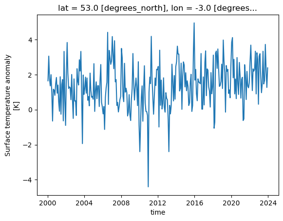
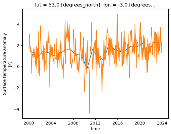
We can plot some data for a single location, across all times in the dataset by using the following:
dataset['tempanomaly'].sel(lat=53, lon=-3).plot()
One thing to note is that Xarray has not only plotted the graph, but has also automatically labelled it based on the long names and units for the variables that were in the metadata of the dataset. The dates on the X axis are also correctly labelled, whereas many plotting libraries require some extra steps to setup labelling dates correctly.
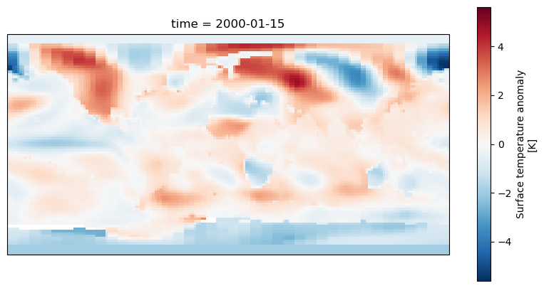
Plotting Two Dimensional Data
Xarray isn’t just restricted to plotting line graphs, if we select some data that returns latitude and longitude dimensions then the plot function will show a map.
dataset['tempanomaly'].sel(time="2000-01-15").plot()
The plot function being called is actually part of the Matplotlib library and we can invoke Matplotlib if we need to modify some of the plotting parameters. For example we might
want to change the colourmap to one which uses grayscale. This can be done by first importing matplotlib.pyplot and specifying the cmap parameter to plot().

import matplotlib.pyplot as plt
dataset['tempanomaly'].sel(time="2000-01-15").plot(cmap=plt.cm.Grays)

Plotting Histograms
Another useful plotting function is to plot a histogram of the data, this could be useful for example to plot the distribution of the temperature anomalies on a given day.
To produce this we call the plot.hist() function on a DataArray.
dataset['tempanomaly'].sel(time="2010-09-15").plot.hist()

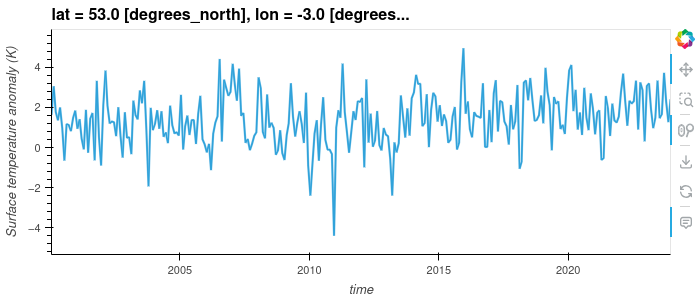
Interactive Plotting with Hvplot
So far we’ve used the matplotlib backend to make our visualisations, this produces some nice graphs but they are completely static and changing the view will require us to change the parameters. Another plotting library we can use is Hvplot, this library allows interactive plots with zooming, panning and displaying the value the mouse is hovering over.
To use hvplot with xarry we must first import the hvplot library with:
import hvplot.xarray
then instead of calling plot() we can now call hvplot().
dataset['tempanomaly'].sel(lat=53,lon=-3).hvplot()
Challenge
Using a slice of the array, plot a transect of the surface temperature anomaly across the Atlantic ocean at 23 degrees North between 70 and 17 degrees West on January 15th 2000 and June 15th 2000.
Solution
dataset['tempanomaly'].sel(time="2000-01-15",lon=slice(-70,-17),lat=23).plot()
dataset['tempanomaly'].sel(time="2000-06-15",lon=slice(-70,-17),lat=23).plot()
Array operations
Map operations
One of the most powerful features of Xarray is the ability to apply a mathematical operation to part or all of an array. Not only is this convienient for us to avoid needing to write one or more for loops to loop over the array applying the operation, it also performs better and can take advantage of some optimsations of our processor. Potentially it can also be parallelised to apply multiple operations simulatenously across different parts of the array, we’ll see more about this later on. These types of operations are known as a “map” operation as they map all the values in the array onto a new of values.
If for example we want to apply a simple offset to our entire dataset we can add or subtract a constant value to every element by doing:
dataset_corrected = dataset['tempanomaly'] - 1.0
Just to confirm this worked, let’s compare the summaries of both datasets:
dataset_corrected
dataset['tempanomaly']
We can combine multiple operations into a single statement if we need to do something more complicated, for example we can apply a linear function by doing:
dataset_corrected = dataset['tempanomaly'] * 1.1 - 1.0
For more complicated operations we might want to write a function and apply that function to the array. Xarray’s Dataset type supports this with its map function,
but map will apply to all variables in the dataset, in the above example we only wanted to apply this to the tempanomaly variable.
There are a couple of ways around this, we could drop the other variables from a copy of the dataset or we can use the apply_ufunc function that works on a single DataArray.
By referencing dataset['tempanomaly'] (or dataset.tempanomaly) we will get hold of a DataArray object that just represents a single variable.
def apply_correction(x):
    x = x * 1.01 + 0.1
    return x

corrected_tempanomaly = dataset.drop_vars("time_bnds").map(apply_correction)
corrected_tempanomaly = xr.apply_ufunc(apply_correction,dataset['tempanomaly'])
We aren’t just restricted to using our own functions with map and apply_ufunc, we can apply any function that can take in a DataArray object. Because of duck typing functions
which take Numpy arrays will also work. For example we can use a function from the Numpy library, one possible function that we might use from Numpy is the clip function, this
requires three arguments, the array to apply the clipping to, the minimum value and maximum value. Any value below the minimum will be converted to the minimum and any value above
the maximum will be converted to the maximum. If for example we wanted to clip our dataset between -2 and +2 degrees then we could do the following:
import numpy
dataset_clipped = xr.apply_ufunc(numpy.clip,dataset['tempanomaly'],-2,2)
Reduce Operations
We’ve now seen map operations that apply a function to every point in an array and return a new array of the same size. Another type of operation is a “reduce” operation which will reduce an array to a single result. Common examples are taking the mean, median, sum, minimum or maximum of an array. Like with map operations, traditionally we might have approached this by using for loops to work through the array and compute the answer. But Xarray allows us to use a single function call to get this result and this has the potential to be parallelised for improved performance.
Both Xarray’s Dataset and DataArray objects have a set of built in functions for common reduce operations including min, max, mean, median and sum.
tempanomaly_mean = dataset['tempanomaly'].mean()
print(tempanomaly_mean.values)
We can also operate on slices of an array, if we wanted to calculate the mean temperature along the transect of 23 degrees North and between 70 and 17 degrees West on January 15th 2000, then we could do:
transect_mean = dataset['tempanomaly'].sel(time='2000-01-15',lon=slice(-70,-17),lat=23).mean()
print(transect_mean.values)
Conditionally Selecting and Replacing Data
Sometimes we want to mask out certain regions of a dataset or to set part of the region to a certain value. Xarray’s where function can be used to replace data based on certain
criteria. There are two (or three depending on how you count) sublety different versions of the where function. One is part of the main Xarray library (e.g. invoked with xr.where)
and it follows the syntax where(cond, x, y), with cond being the condition to apply, x being what to do if it is true and y if it is false. The other version of the where function
exists in the xarray.DataArray and xarray.Dataset packages and has a slightly different syntax of where(cond, other), here other refers to what do when the condition is false,
if the condition is true then the value currently in this position is copied to the resulting array and if other is not specified the value is converted to an NaN (not a number).
For example if we want all data that is negative to be converted to an NaN then we could use the Dataset/DataArray version of where:
dataset['tempanomaly'].where(dataset['tempanomaly'] >= 0.0)
If we decided that we wanted to make all negative values zero and multiply all positive values by 2 then we could use the xr.where function instead,
xr.where(dataset['tempanomaly'] < 0.0, 0, dataset['tempanomaly'] * 2.0)
The DataArray version of where can also apply conditions against dimensions instead of variables, for example if we wanted to mask out all of the Western hemisphere values with NaNs
then we could use:
dataset['tempanomaly'].where(dataset['tempanomaly'].lon > 0)
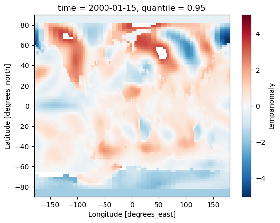
Challenge
Using map/reduce operations and the where function to do the following on the example dataset:
- Calculate the 95th percentile of the data set using the
quantilefunction in Xarray.- Use the where function to remove any data above the 95th percentile.
- Multiply all remaining values by a correction factor of 0.90.
- Plot both the original and corrected version of the dataset for the first day in the dataset (2000-01-15).
Solution
threshold = dataset['tempanomaly'].quantile(0.95)
lower_95th = dataset['tempanomaly'].where(dataset['tempanomaly'] < threshold)
lower_95th = lower_95th * 0.90
lower_95th[0].plot()
# do this in a different Jupyter cell or you only get one plot
dataset['tempanomaly'][0].plot()
Xarray Patterns
Computational patterns are common operations that we might perform. Xarray has several patterns that it recommends and has been designed to faciliate. These include:
- Resampling
- Grouping Data
- Rolling Windows
- Coarsening
Resampling
Xarray can resample data to reduce its frequency, this is done through the resample function on a DataArray or Dataset. Resample only works on the time dimension of a dataset/array.
Let’s call resample on a selection of our data for a single location, we can then produce a line graph of the temperature over time and see the difference between the original and
resampled version. The resample function takes a paramter of a variable name mapped (with the = symbol) to a resampling frequency, this could be “h” for hourly, “D” for daily, “W”
for weekly, “ME” for month endings, “MS” for month starts, “YS” for year starts and “YE” for year ends. These options are borrowed from the Pandas resample frequency and a full list
of them can be found in the Pandas documentation. In our example we’ll do a yearly resampling,
since the data is already monthly.
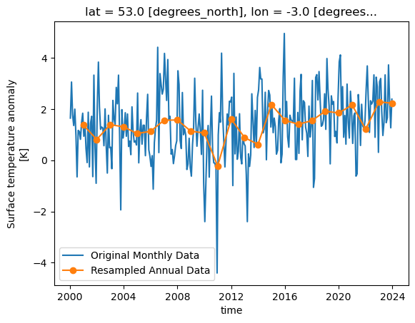
resampled = dataset['tempanomaly'].sel(lat=53,lon=-3).resample(time="1YE")
This will return a DataArrayResample object that details the resampling, but we haven’t actually resampled yet. To do that we have to apply an averaging function such as mean to
the DataArrayResample object. We can apply this and plot the result, for comparison let’s plot the original data alongside it too. To get a legend we need to import matplotlib.pyplot
and call it’s legend function.
import matplotlib.pyplot as plt
dataset['tempanomaly'].sel(lat=53,lon=-3).plot(label="Original Monthly Data")
resampled.mean().plot(label="Resampled Annual Data",marker="o")
plt.legend()
Group by
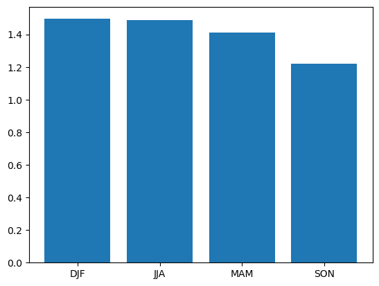
The group by pattern allows us to group related data together, a common example in environmental science is to group monthly data into seasonal groups of three months each.
We can group these by calling the groupby function and specifying that we want the data in seasonal groups with “time.season” as the parameter to groupby. If we had
daily data and wanted it grouped by months then we could use “time.month” instead.
grouped = dataset['tempanomaly'].sel(lat=53,lon=-3).groupby("time.season")
In a similar way to how resample returned a DataArrayResample object, groupby returns a DataArrayGroupBy object that describes the groups we’ve created, but we need to apply some kind
of reduce operation to bring any data into these groups. Again, applying a mean makes sense here to produce a mean value for each season. As there are only four of these lets plot them
as a bar chart, we need to give the names of the groups and the values we’ll be plotting to plt.bar.
grouped_mean = grouped.mean()
plt.bar(grouped_mean.season,grouped_mean)
Binned Group By
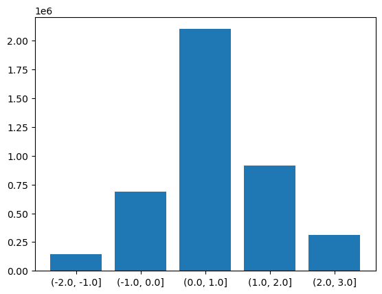
There is another version of the groupby function called groupby_bins which allows us to group data into bins covering a range of values.
bins = [-2.0,-1.0,0.0,1.0,2.0,3.0]
binned = dataset.groupby_bins("tempanomaly",bins)
Again as with our other functions we get an object back from groupby_bins that defines the bins, but doesn’t put any data onto them. In this case lets find out how many items are in each bin by using the count function to count them.
counts = binned.count()
Now to display this on a graph requires a bit of processing to extract the labels of the bins, we need to loop through all the bins and convert their names into strings. Once this is done we can plot a bar graph showing the counts in each bin.
labels = []
for i in range(0,len(counts['tempanomaly'])):
    print(counts['tempanomaly_bins'][i].values,counts['tempanomaly'][i].values)
    labels.append(str(counts['tempanomaly_bins'][i].values))

plt.bar(labels,counts['tempanomaly'].values)
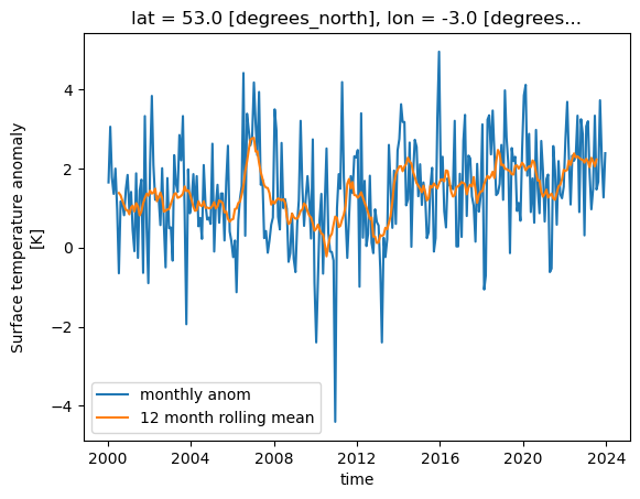
Rolling Windows
Xarray can work on a “rolling window” of data that covers a subset of the data. This can be useful for example to calculate a rolling mean of 12 months worth of data. The following will graph both the monthly values and the rolling mean temperature anomaly for Liverpool, UK.
import matplotlib.pyplot as plt

rolling = dataset['tempanomaly'].rolling(time=12, center=True)
ds_rolling = rolling.mean()
dataset.tempanomaly.sel(lon=-3, lat=53).plot(label="monthly anom")
ds_rolling.sel(lon=-3,lat=53).plot(label="12 month rolling mean")
plt.legend()
Coarsening
Coarsening can be used to reduce the resolution of data in a similar way to resample. The difference is that the Xarray coarsen function specifies the interval it works
across. If data is missing then coarsen will take account of that, while resample will not.
coarse = dataset.coarsen(lat=5,lon=5, boundary="trim")
This will return a DataCoarsen object that represents 5 degree windows across the lat and lon dimensions of the dataset.
To do something useful with it we need to apply a function such as mean that will calulate a new dataset/array using our coarsening operation.
coarse.mean()['tempanomaly'][0].plot()
We aren’t just restricted to working across spatial dimensions, coarsening can also operate in time, for example to convert a monthly dataset to an annual one.
coarse = dataset.coarsen(time=12)
coarse.mean()['tempanomaly'].sel(lat=53,lon=-3).plot()
#for comparison
dataset['tempanomaly'].sel(lat=53,lon=-3).plot()
Writing Data
Once we have finished calculating some new data with Xarray we might want to write it back to a NetCDF file. Using the earlier example of a dataset which has had some corrections applied, we could write this data back to a NetCDF file by doing:
dataset_corrected = dataset['tempanomaly'] * 1.1 - 1.0
dataset_corrected.to_netcdf("corrected.nc")
Challenge
There are several example datasets built into Xarray. You can load them with the
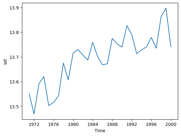
tutorial.load_datasetfunction from the main xarray library. One of these is the Extended Reconstructed Sea Surface Temperature data from NOAA, known as “ersstv5”. Load this data with Xarray and do the following:
- Slice the data so that only data from before 2000 is included, by defalt the dataset runs up to the end of 2021.
- Resample the data to annual means.
- Calculate a global annual mean for each year.
- Plot the global mean temperatures on a line graph.
- Write the resulting Dataset to a new NetCDF file.
Solution
import xarray as xr
sst = xr.tutorial.load_dataset("ersstv5")
sst_20c = sst.sel(time=slice("1970-01-01","1999-12-31"))
sst_annual = sst_20c.resample(time="1YE").mean()
sst_global = sst_annual.mean(dim=['lat','lon'])
#sst_global = sst_annual.coarsen(lat=89,lon=180).mean() #another way to do the same as above
sst_global['sst'].plot()
sst_global.to_netcdf("global-mean-sst.nc")
Key Points
Xarray can load NetCDF files
We can address dimensions by their name using the
.dimensionname,['dimensionname]orsel(dimensionname)syntax.With lazy loading data is only loaded into memory when it is requested
We can apply mathematical operations to the whole (or part) of the array, this is more efficient than using a for loop.
We can also apply custom functions to operate on the whole or part of the array.
We can plot data from Xarray invoking matplotlib.
Hvplot can plot interactive graphs.
Xarray has many useful built in operations it can perform such as resampling, coarsening and grouping.
Plotting Geospatial Data with Cartopy
Overview
Teaching: 30 min
Exercises: 20 minQuestions
How do I plot data on a map using Cartopy?
Objectives
Understand the need to choose appropriate map projections
Apply cartopy to plot some data on a map
Plotting Data with Cartopy
We have seen some basic plots created with Xarray and Matplotlib, but when plotting data on a map this was restricted to quite a simple 2D map without any labels or outlines of coastlines or countries. The Cartopy library allows us to create high quality map images, with a variety of different projections, map styles and showing the outlines of coasts and country boundaries.
Using Xarray data with Cartopy
To plot some Xarray data from our example dataset we’ll need to select a single day (or combine multiple days together). As Cartopy can work with array types such as Numpy arrays it will also work with Xarray arrays.
Let’s start a new notebook and do some initial setup to import xarray, cartopy and we’ll also need matplotlib since Cartopy uses it.
import xarray as xr
import cartopy.crs as ccrs
import matplotlib.pyplot as plt
dataset = xr.open_dataset("gistemp1200-21c.nc")
To setup a Cartopy plot we’ll need to create a matplotlib figure and add a subplot to it. Cartopy also requires us to specify a map projection, for this example we’ll use the PlateCarree
projection. Note that due to how Matplotlib interacts with Jupyter notebooks, the following must all appear in the same cell.
To extract some data from our datset we’ll use dataset['tempanomaly'].sel(time="2000-01-15") to get the temperature anomaly data for January 15th 2000.
fig = plt.figure(figsize = (10, 5))
axis = fig.add_subplot(1, 1, 1, projection = ccrs.PlateCarree())
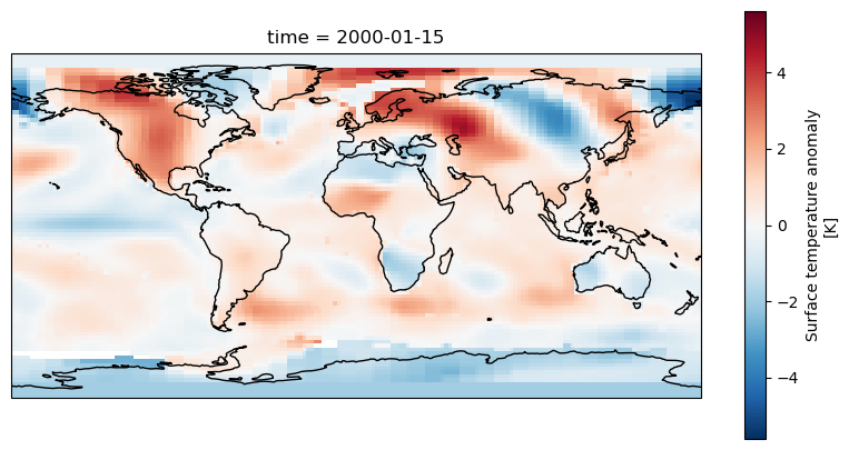
dataset['tempanomaly'].sel(time="2000-01-15").plot(ax = axis)
We should now see a map of the world with the temperature anomaly data, if we look in the top left we can see North America appearing mostly in red and in the lower right Australia in blue,
but much of the other continents are harder to make out. To make it easier we can add coastlines by calling axis.coastlines() after the plot. But to make this appear on the same map
as the rest of the plot it needs to be in the same Jupyter cell and we’ll have to rerun the whole cell.
fig = plt.figure(figsize = (10,5))
axis = fig.add_subplot(1, 1, 1, projection = ccrs.PlateCarree())
dataset.tempanomaly.sel(time="2000-01-15").plot(ax = axis)
axis.coastlines()
Dealing with Projections
Cartopy supports many different map projections which change how the globe is mapped onto a two dimensional surface. This is controlled by the projection parameter to fig.add_subplot.
One alternative projection we can use is the RotatedPole projection which will project the pole at the centre of the map, this takes two parameters pole_latitude and pole_longitude
which define the point at which we want to centre the map on.
fig = plt.figure(figsize=(10,5))
axis = fig.add_subplot(1, 1, 1, projection=ccrs.RotatedPole(pole_longitude=-90, pole_latitude=0))
dataset.tempanomaly.sel(time="2000-01-15").plot(ax = axis)
axis.coastlines()
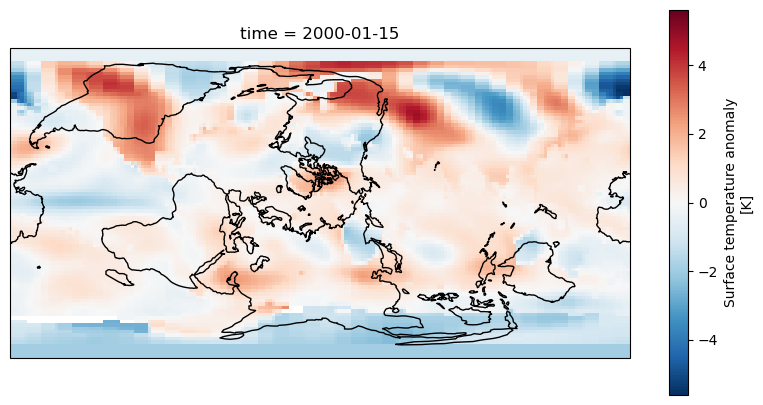
The above example puts the map into a RotatedPole projection, but notice that the coastlines and coloured areas of the map don’t match as they previously did. This is because
we haven’t told Cartopy how the data is structured and it has assumed it matches the projection. We didn’t need to do this with the PlateCarree projection as the data matched the projection
but now we need to specify an extra transform argument to plot.
fig = plt.figure(figsize=(10,5))
axis = fig.add_subplot(1, 1, 1, projection=ccrs.RotatedPole(pole_longitude=-90, pole_latitude=0))
dataset.tempanomaly.sel(time="2000-01-15").plot(ax = axis, transform=ccrs.PlateCarree())
axis.coastlines()
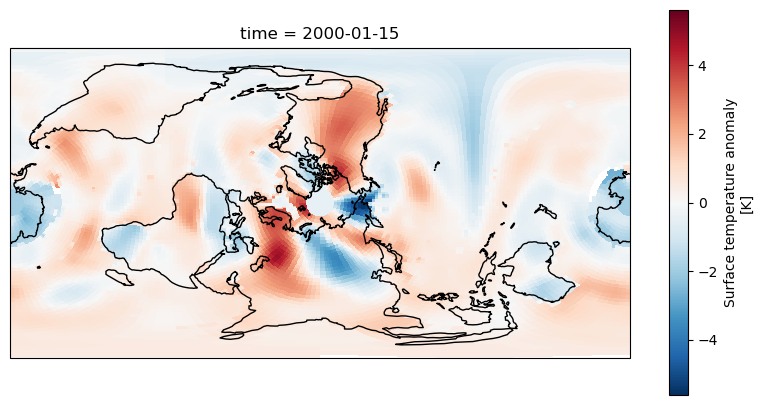
The data should now match the coastlines.
Challenge
Experiment with the following map projections
- Mollweide
- InterruptedGoodeHomolosine
- Robinson
- Orthographic (requires latitude and longitue parameters) See https://scitools.org.uk/cartopy/docs/v0.13/crs/projections.html for more options. Which do you like the most? Discuss what is the most useful aspects for showing data with the group.
Adding gridlines
Like we added coastlines with axis.coastlines() we can add gridlines of latitude and longitude with axis.gridlines(). By default these will appear every 60 degrees of longitude and
every 30 degrees of latitude. We can add labels with the parameter draw_labels=True.
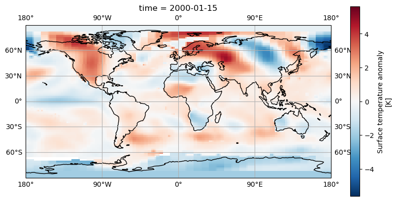
fig = plt.figure(figsize=(10,5))
axis = fig.add_subplot(1, 1, 1, projection=ccrs.PlateCarree())
dataset.tempanomaly.sel(time="2000-01-15").plot(ax = axis, transform=ccrs.PlateCarree())
axis.coastlines()
axis.gridlines(draw_labels=True)
If we’d like the gridlines at a different position we can specify these with Python lists in the xlocs and ylocs parameters. For example
fig = plt.figure(figsize=(10,5))
axis = fig.add_subplot(1, 1, 1, projection=ccrs.PlateCarree())
dataset.tempanomaly.sel(time="2000-01-15").plot(ax = axis, transform=ccrs.PlateCarree())
axis.coastlines()
axis.gridlines(draw_labels=True,xlocs=[-180,-90,0,90,180])
A more concise way to do this is to use Numpy’s linspace function which creates an array of evenly spaced elements, this takes a start, end and number of elements parameter for example:
axis.gridlines(draw_labels=True,xlocs=np.linspace(-180,180,5))
Adding Country/Region boundaries
Cartopy has many common map features including coastlines, lakes, rivers, country boundaries and state/region boundaries that it can draw. These are all available in the cartopy.feature
library and can be added using the add_features function on a subplot axis.
import cartopy.feature as cfeature
fig = plt.figure(figsize=(10,5))
axis = fig.add_subplot(1, 1, 1, projection=ccrs.PlateCarree())
dataset.tempanomaly.sel(time="2000-01-15").plot(ax = axis, transform=ccrs.PlateCarree())
axis.coastlines()
axis.gridlines(draw_labels=True)
axis.add_feature(cfeature.BORDERS)
axis.add_feature(cfeature.LAKES)
axis.add_feature(cfeature.RIVERS)
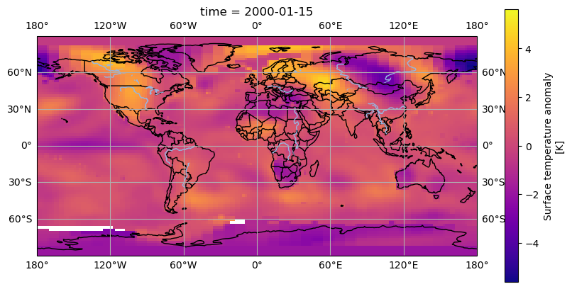
The above code will add country boundaries, lakes and rivers to our map. The lakes and rivers might be a little hard to see in places where there is a blue being used to render the temperature anomaly. We could apply a different colourmap to avoid this problem, the plasma colourmap in Matplotlib goes from purple, to orange to yellow and shows the contrast with the rivers nicely.
from matplotlib import colormaps
fig = plt.figure(figsize=(10,5))
axis = fig.add_subplot(1, 1, 1, projection=ccrs.PlateCarree())
dataset.tempanomaly.sel(time="2000-01-15").plot(ax = axis, transform=ccrs.PlateCarree(), cmap=colormaps.get_cmap('plasma'))
axis.coastlines()
axis.gridlines(draw_labels=True)
axis.add_feature(cfeature.BORDERS)
axis.add_feature(cfeature.LAKES)
axis.add_feature(cfeature.RIVERS)
Downloading boundary data manually
If you want to download the boundary data yourself (perhaps if you are going to be offline later and want to plot some maps) then you can do this from the Natural Earth website or by using a wget or curl command from your terminal. Download the following files:
- https://naturalearth.s3.amazonaws.com/110m_physical/ne_110m_coastline.zip
- https://naturalearth.s3.amazonaws.com/110m_physical/ne_110m_lakes.zip
- https://naturalearth.s3.amazonaws.com/110m_physical/ne_110m_rivers_lake_centerlines.zip
- https://naturalearth.s3.amazonaws.com/110m_cultural/ne_110m_admin_0_boundary_lines_land.zip
Unzip these and place the coastlines, lakes and rivers files in
~/.local/share/cartopy/shapefiles/natural_earth/physical.Place the boundaries in
~/.local/share/cartopy/shapefiles/natural_earth/culturalCartopy also includes a script called
cartopy_feature_downloadwhich can download these files for you and place them in the correct location.Here’s the commands to do all of this using Cartopy’s script:
cartopy_feature_download physical --output  ~/.local/share/cartopy/shapefiles/natural_earth/physical
cartopy_feature_download gshhs --output  ~/.local/share/cartopy/shapefiles/natural_earth/physical
cartopy_feature_download cultural --output  ~/.local/share/cartopy/shapefiles/natural_earth/cultural
cartopy_feature_download cultural-extra --output  ~/.local/share/cartopy/shapefiles/natural_earth/cultural
Manual method:
wget https://naturalearth.s3.amazonaws.com/110m_physical/ne_110m_coastline.zip https://naturalearth.s3.amazonaws.com/110m_physical/ne_110m_lakes.zip https://naturalearth.s3.amazonaws.com/110m_physical/ne_110m_rivers_lake_centerlines.zip https://naturalearth.s3.amazonaws.com/110m_cultural/ne_110m_admin_0_boundary_lines_land.zip
mkdir -p ~/.local/share/cartopy/shapefiles/natural_earth/cultural
mkdir -p ~/.local/share/cartopy/shapefiles/natural_earth/physical
cd ~/.local/share/cartopy/shapefiles/natural_earth/cultural
conda run -n esces unzip ~/ne_110m_admin_0_boundary_lines_land.zip
cd ../physical
conda run -n esces unzip ~/ne_110m_coastline.zip
conda run -n esces unzip ~/ne_110m_lakes.zip
conda run -n esces unzip ~/ne_110m_rivers_lake_centerlines.zip
Challenge
The
cartopy.feature.NaturalEarthFeaturelibrary allows access to a number of boundary features from the shapefiles supplied by the website Natural Earth. One of these has administrative and state boundaries for many countries. Add this feature using the “admin_1_states_provinces_lines” dataset. Use the 50m (1:50 million) scale for this.Solution
states_provinces = cfeature.NaturalEarthFeature(
       category='cultural',
       name='admin_1_states_provinces_lines',
       scale='50m',
       facecolor='none')
axis.add_feature(states_provinces)
Key Points
Cartopy can plot data on maps
Cartopy can use Xarray DataArrays
We can apply different projections to the map
We can add gridlines and country/region boundaries
Coffee Break
Overview
Teaching: min
Exercises: minQuestions
Objectives
Feedback
In the etherpad, answer the following questions:
- Are we going too fast, too slow or just write? Record your answer in the etherpad
- What’s the most useful thing we’ve covered so far?
- What don’t you understand or would like clarification on?
Take a break!
- Drink something
- Eat something
- Talk to each other
- Get some fresh air
Key Points
Parallelising with Dask
Overview
Teaching: 50 min
Exercises: 30 minQuestions
How do we setup and monitor a Dask cluster?
How do we parallelise Python code with Dask?
How do we use Dask with Xarray?
Objectives
Understand how to setup a Dask cluster
Recall how to monitor Dask’s performance
Apply Dask to work with Xarray
Apply Dask futures and delayed tasks
What is Dask?
Dask is a Distributed processing library for Python. It enables parallel processing of Python code across multiple cores on the same computer or across multiple computers. It can be used behind the scenes by Xarray with minimal modification to code. JASMIN users can make use of a Dask gateway that allows their Dask code submitted from the Jupyter notebook interface to run on the Lotus HPC cluster. Dask has two broad categories of features, high level data structures which behave in a similar way to common Python data structures but with the ability to perform operations in parallel and low level task scheduling to run any Python code in parallel.
Setting up Dask on your computer
Dask should already be installed in your Conda/Mamba environment. Dask refers to the system it runs the computation on as a Dask “cluster”, although the “cluster” can just be running on your local computer (or the JASMIN notebook server). Later on we’ll look at using a remote cluster running on a different computer, but for now let’s create one on our own computer.
from dask.distributed import Client, progress
client = Client(processes=False, threads_per_worker=4,
                n_workers=1, memory_limit='2GB')
client
The code above will create a local Dask cluster with one worker and 4 threads for each worker and a limit of 2GB of memory. Displaying the client object will tell us all about the
cluster.

Using the Dask dashboard
In the information about the Dask cluster is a link to a Dashboard webpage. From the Dashboard we can monitor our Dask cluster and see how busy it is, view a graph of task dependencies, memory usage and the status of the Dask workers. This can be really useful when checking if our Dask cluster is behaving correctly and working out how optimially our code is making use of Dask’s parallelism.
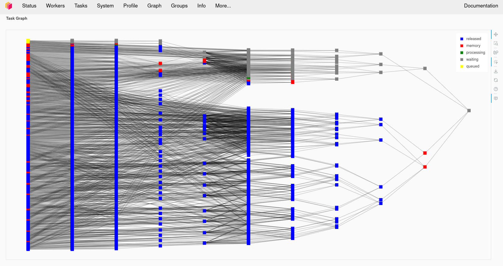
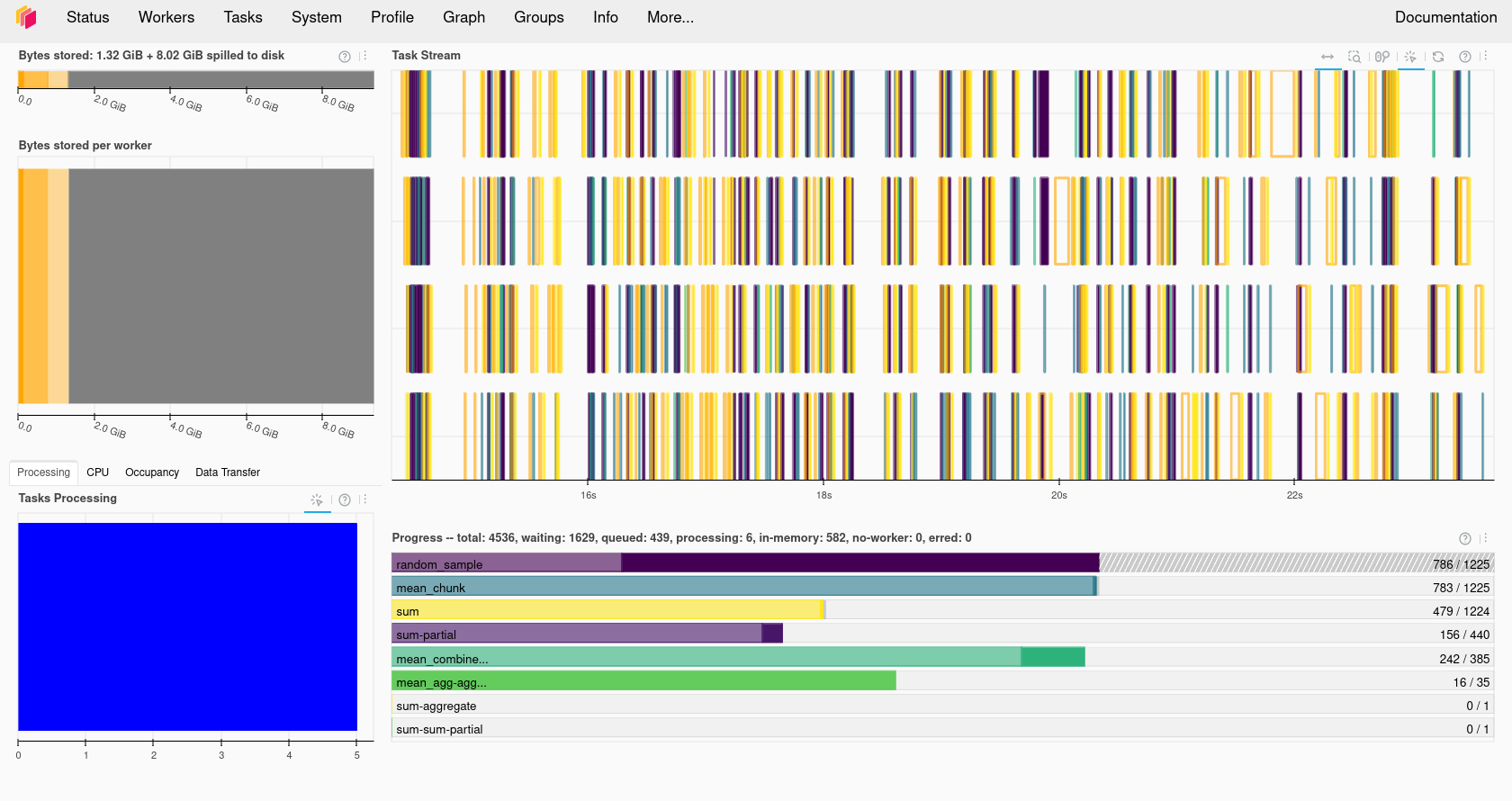
Using the Dask dashboard on JASMIN
Note that if you are using the JASMIN notebook service, the link to the dashboard won’t work as the port it runs on isn’t open to connections from the internet.
ssh-keygen #MAKE SURE YOU SET A PASSPHRASE
cat ~/.ssh/id_rsa.pub >> ~/.ssh/authorized_keys
ssh -R 8788:localhost:8787 login-02.jasmin.ac.uk
Port 8787 might not be the port your Dask cluster is using, make sure the first 8787 is the number your Dask cluster is running on. If anybody else is doing this then port 8788 on login-02 might be in use, change the second 8788 to something else to match. Now connect an SSH tunnel from your computer to Jasmin login-02 and forward port 8788 back to your computer where it will be presented as port 8789.
ssh -L 8789:localhost:8788 login-02.jasmin.ac.uk
Open your web browser to http://127.0.0.1:8789 and you will see your Dask cluster page. Note that you have just exposed this to anybody else with JASMIN access and there is no password on it.
Dask Arrays
Dask has its own type of arrays, these behave much like Numpy (and Xarray) arrays, but they can be split into a number of chunks. Any processing operations can work in parallel across these chunks. Data can also be loaded “lazily” into Dask Arrays, this means it is only loaded from disk when it is accessed. This can give us the illusion of loading a dataset that is larger than our memory.
Creating a Dask Array
Dask arrays can be created from existing from other array formats including NumPy arrays, Python lists and PandasDataFrames.
We can also initalise a new array as a Dask Array from the start, Dask copies the zeros, ones and random functions from NumPy which initalise an array as all zeros, ones or as
random numbers. For example to create a 10000x10000 array of random numbers we can use:
import dask.array as da
x = da.random.random((10000, 10000), chunks=(1000, 1000))
x
Dask arrays support common Numpy operations including slicing, arithmetic whole array operations, reduction functions such as mean and sum, transposing and reshaping.
y = da.ones((10000,10000), chunks = (1000, 1000))
z = x + y
z
In the above example we added the x and y arrays together, but when we display the result we just get an array getitem in response instead of an actual value. This is because Dask
hasn’t actually computed the result yet. Dask works by building up a dependency graph of all the operations we’re performing, but doesn’t compute anything until we call the compute
function on the final result. Let’s go ahead and call compute on the z object, if we monitor the Dask Dashboard we should see some activity.
result = z.compute()
result
The new variable result will now contain the result of the computation and will be of the type numpy.ndarray.
type(result)
Compare Dask and Numpy Performance
Compare the performance of the following code using Numpy and Dask functions. Use the %%time magic in the cells to find out the execution time. Ensure you only time the core computation and not the Dask cluster setup or library imports, this means you’ll have to write this code into multiple cells. Dask version (note you’ll need to do the Dask client setup first):
import dask.array as da
x = da.random.random((20000,20000), chunks=(1000,1000))
x_mean = x.mean()
x_mean.compute()
Numpy version:
import numpy as np
npx = np.random.random((20000,20000))
npx_mean = npx.mean()
Which went faster overall? Why do you think you got the result you did? Try making the dataset a little larger, going much beyond 25000x25000 might use too much memory. Try running the
topcommand in a terminal while your notebook is running, look at the CPU % when running the Numpy and Dask versions and compare them. Try changing the number of Dask threads and see what effect this has on the CPU %.
Troubleshooting Dask
Sometimes Dask can jam up and stop executing tasks. If this happens try the following:
- Shutdown the client and restart it.
- Shutdown the kernel of your notebook and rerun the notebook.
Using Dask with Xarray
We previously used Xarray to load our temperature anomaly dataset from the Goddard Institute for Space Studies and performed some computational operations against it using Xarray.
Let’s go and load it again, but this time we’ll give an extra option to open_dataset, the chunk option which allows us to chunk the Xarray data to prepare it for computing with Dask.
The chunk option expects a Python dictionary defining the chunk size for each of the dimensions, any dimension we don’t want to chunk should be set to -1. For example:
import xarray as xr
from dask.distributed import Client
client = Client(n_workers=2, threads_per_worker=2, memory_limit='1GB')
client
ds = xr.open_dataset("gistemp1200-21c.nc", chunks={'lat':30, 'lon':30, 'time':-1})
ds
da = ds['tempanomaly']
da
Here we see that the Dask DataArray da is now chunked every 30 degrees of Latitude and Longitude. We can also specify automatic chunking by using chunks={}, but with such a small
dataset there won’t be any chunking applied automatically.
Any Xarray operations we now apply to the array will now use Dask. Let’s repeat some of our earlier Xarray examples and compute a correction factor to the dataset, if we watch the Dask dashboard we’ll see some signs of activity.
dataset_corrected = ds['tempanomaly'] * 1.1 - 1.0
If we print dataset_corrected we’ll see that it actually contains a Dask array.
print(dataset_corrected)
Dask is “lazy” and doesn’t compute anything until we tell it to. To get Dask to trigger computing the result we need to call .compute on dataset_corrected.
result = dataset_corrected.compute()
result
Low Level computation with Dask
When higher level Dask functions are not sufficient for our needs we can write our own functions and request Dask executes these in parallel. Dask has two different strategies we can use
for this, Delayed functions and Futures. Delayed functions will delay starting until we call .compute at which point all the dependencies of the operation we request are executed.
With futures tasks begin as soon as possible and immediately return a future object that is eventually populated with the result when the operation completes.
Delayed Tasks
To execute a function as a delayed task we must tag it with a dask.delayed decorator. Here is a simple example:
import dask
@dask.delayed
def apply_correction(x):
   return x * 1.01 + 0.1

import dask.array as da
x = da.random.random(1_000_000, chunks=1000)
corrected = apply_correction(x)

squared = corrected ** 2

result = squared.compute()
This will call the apply_correction function on each of the 1000 chunks that make up the array x and then square the result. But nothing will execute until we call the compute
function on the last line. Both squared and corrected will have the type of dask.delayed.Delayed until they have been computed.
Visualising the Task Graph
We have already seen that we can visualise the Dask task graph in the dashboard as it is executing. But we can also visualise it inside a Jupyter notebook by calling the visualize
function on a Dask datastructure. We can render this before we call compute if we want to see what is going to happen. This may not always work with larger datasets, our example above
with 1,000,000 elements and 1000 chunks is going to be too big, but if we reduce the size of the array x to 10,000 items instead of 1,000,000 then it will be possible.
@dask.delayed
def apply_correction(x):
   return x * 1.01 + 0.1

import dask.array as da
x = da.random.random(10_000, chunks=1000)
corrected = apply_correction(x)

squared = corrected ** 2

squared.visualize()

result = squared.compute()
Futures
An alternative approach to using any function with Dask is to use Dask Futures. These begin execution immediately, but are non-blocking so execution (appears to) proceeds to the next statement while the processing is done in the background. Any objects which are returned by a function will have a Dask future type until the exectuion has completed.
If we want to block until a result is available then we can call the result function. For example taking the code from the last section we can do the following:
import dask.array as da

def apply_correction(x):
   return x * 1.01 + 0.1

def square(x):
   return x ** 2

x = da.random.random(10_000, chunks=1000)
corrected = client.submit(apply_correction, x)

corrected

squared = client.submit(square, corrected)

squared

squared = squared.result()
squared
If we watch the task activity in the Dask dashboard then we should see activity start as soon as the client.submit calls are made. The squared and corrected variables
will be Dask future objects, if we display them we will see their status as to whether they are finished or not.
When to use Futures or Delayed
The Dask documentation does not have much advice on when it is more appropriate to use Futures or Delayed functions. Some general advice from the forums is to use Delayed functions and task graphs first, but to switch to futures for more complicated problems.
Using the JASMIN Dask gateway
JASMIN offers a Dask Gateway service which can submit Dask jobs to a special queue on the Lotus cluster. To use this we need to do a bit of extra setup. We will need to import
the dask_gateway library and configure the gateway.
import dask_gateway
gw = dask_gateway.Gateway("https://dask-gateway.jasmin.ac.uk", auth="jupyterhub")
The gateway can be given a set of options including how many worker cores to use, initially we can set this to one and scale it up later. We also need to allocate at least one core
as to the scheduler which will manage our Dask cluster. JASMIN requires us to specify a project to associate the Dask jobs with.
You can find out which projects you are a member of by running the command useraccounts on a sci server. If you are not a member of any project then you can
use “no-project” here, but if you are a member of a project you must use a project name. Finally we need to tell Dask which Conda/Mamba environment to use and this needs to match the one we’re running in our notebook.
options = gw.cluster_options()
options.worker_cores = 1
options.scheduler_cores = 1
options.account = "no-project"
options.worker_setup='source /apps/jasmin/jaspy/miniforge_envs/jaspy3.11/mf3-23.11.0-0/bin/activate ~/.conda/envs/esces'
Finally we can check if we already had a cluster running and reuse that if we do and then get a client object from the cluster that will behave
the same way as the local Dask client did.
clusters = gw.list_clusters()
if not clusters:
    cluster = gw.new_cluster(options, shutdown_on_close=False)
else:
    cluster = gw.connect(clusters[0].name)

client = cluster.get_client()
Now that we have a running cluster we can allow it to adapt and scale up and down as we demand it. This will translate to Slurm jobs being launched on the JASMIN cluster itself. JASMIN allows users to spawn up to 16 jobs in the Dask queue, but one of these will be taken by the scheduler so the we can only launch a maximum of 15 workers.
cluster.adapt(minimum=1, maximum=15)
If we now connect to one of the JASMIN sci servers (sci-vm-01 to 05 or sci-ph-01 to 03) we can see our jobs in the SLURM queue by running the squeue command.
ssh -J <jasminusername>@login-02.jasmin.ac.uk <jasminusername>@sci-vm-03
squeue -p dask
Once we are done with Dask we can shutdown the cluster by calling its shutdown function. This should cause the jobs in the SLURM queue to finish.
cluster.shutdown()
JASMIN Dask Dashboard
If you display the contents of the client or cluster variable then you will be given an address beginning https://dask-gateway.jasmin.ac.uk that will take you to a Dask
dashboard for your cluster. Unfortunately this server is only accessible within the JASMIN network, to access it you will have to use a web browser running inside an
NoMachine session or port forward via the JASMIN login server.
Challenge
Setup Dask a Dask cluster on JASMIN. Load the GIS temperature anomaly dataset with Xarray and run the correction algorithm on it. Time how long the compute operation takes by using the %%time magic. Experiment with:
- Changing the chunk sizes you use in Xarray
- Changing the number of worker cores
- Changing the number of workers (set in
cluster.adapt)Solution
import dask_gateway
import xarray as xr
print(dask_gateway.__version__)
# Create a connection to dask-gateway.
gw = dask_gateway.Gateway("https://dask-gateway.jasmin.ac.uk", auth="jupyterhub")

options = gw.cluster_options()
options.worker_cores = 2
options.scheduler_cores = 1
options.account = "no-project"
options.worker_setup='source /apps/jasmin/jaspy/miniforge_envs/jaspy3.11/mf3-23.11.0-0/bin/activate ~/.conda/envs/esces'
clusters = gw.list_clusters()
if not clusters:
    cluster = gw.new_cluster(options, shutdown_on_close=False)
else:
   cluster = gw.connect(clusters[0].name)
client = cluster.get_client()
cluster.adapt(minimum=1, maximum=4)
ds = xr.open_dataset("gistemp1200-21c.nc", chunks={'lat':30, 'lon':30, 'time':-1})
ds
da = ds['tempanomaly']
da
dataset_corrected = ds['tempanomaly'] * 1.1 - 1.0
print(dataset_corrected)
cluster.shutdown()
Key Points
Dask is a parallel computing framework for Python
Dask creates a task graph of all the steps in the operation we request
Dask can use your local computer, an HPC cluster, Kubernetes cluster or a remote system over SSH
We can monitor Dask’s processing with its dashboard
Xarray can use Dask to parallelise some of its operations
Delayed tasks let us lazily evaluate functions, only causing them to execute when the final result is requested
Futures start a task immediately but return a futures object until computation is completed
Lunch Break
Overview
Teaching: min
Exercises: minQuestions
Objectives
Feedback
In the etherpad answer the following questions:
- Are we going too fast, too slow or just write? Record your answer in the etherpad
- What’s the most useful thing we’ve covered so far?
- What don’t you understand or would like clarification on?
Have some lunch
- Take a break
- Eat something
- Drink something
- Talk to each other
- Get some fresh air
Key Points
Storing and Accessing Data in Parallelism Friendly Formats
Overview
Teaching: 50 min
Exercises: 30 minQuestions
How is the performance of data access impacted by bandwidth and latency?
How can we use an object store to store data that is accessible over the internet?
How do we access data in an object store using Xarray?
Objectives
Understand the relative performance of memory, local disks, local networks and the internet.
Understand that object stores are a convienient and scalable way to store data to be accessed over the internet.
Understand how Zarr files can be structured in an object store friendly way.
Apply Xarray to access Zarr files stored in an object store.
Data Access Speeds
The time spent accessing data from disk is orders of magnitude more than accessing data stored in RAM and accessing data over a network is orders of magnitude more than accessing data on a local disk. This is visualised nicely in the diagram below
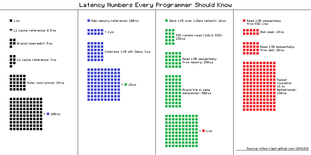
(from https://gist.github.com/hellerbarde/2843375)
Lets multiply all these durations by a billion:
Magnitudes:
Minute:
- L1 cache reference 0.5 s One heart beat (0.5 s)
- Branch mispredict 5 s Yawn
- L2 cache reference 7 s Long yawn
- Mutex lock/unlock 25 s Making a coffee
Hour:
- Main memory reference 100 s Brushing your teeth
- Compress 1K bytes with Zippy 50 min One episode of a TV show (including ad breaks)
Day:
- Send 2K bytes over 1 Gbps network 5.5 hr From lunch to end of work day
Week
- SSD random read 1.7 days A normal weekend
- Read 1 MB sequentially from memory 2.9 days A long weekend
- Round trip within same datacenter 5.8 days A medium vacation
- Read 1 MB sequentially from SSD 11.6 days Waiting for almost 2 weeks for a delivery
Year
- Disk seek 16.5 weeks A semester in university
- Read 1 MB sequentially from disk 7.8 months Almost producing a new human being
- The above 2 together 1 year
Decade
- Send packet CA->Netherlands->CA 4.8 years Average time it takes to complete a bachelor’s degree
We are going to have to wait a really long time to get data from the internet when compared to processing it locally. But in the modern era when we might be working with multiterabyte (or even petabyte) datasets it isn’t likely to be practical to store it all on our local computer. By applying parallel working patterns we can also have multiple computers each compute part of a dataset and/or we can have multiple computers each store part of the dataset allowing us to transfer several parts of it in parallel.
Parallel Filesystems
On many high performance computing (HPC) systems it is common for there to be a large parallel filesystem. These will spread data across a large number of physical disks and servers, when a user requests some data it might be supplied by several servers simultaneously. Since each disk can only supply data so fast (usually between 10s and 100s of megabytes per second) we can achieve faster data access by requesting from several disks spread across several servers. Many parallel filesystems will be configured to provide access speeds of multiple gigabytes per second. However HPC systems also tend to be shared systems with many users all running different tasks at any given time, so the activities of other users will also impact how quickly we can access data.
Object Stores
Object stores are a scalable way to store data in a manner that is readily accessible over the internet. They use the Hyper Text Transfer Protocol (HTTP) or its secure alternatie (HTTPS) to access “objects”. In this case each object will have a unique URL and the appearance of a file on a filesystem. Where object stores differ from traditional filesystem is that there isn’t any directory hierarchy to the objects, although sometimes object stores are configured to give the illusion of this. For example we might create object names that contain path separators. The underlying storage can “stripe” the data of an object across several disks and/or servers to achieve higher throughput speeds in a similar way to the parallel filesystems described above, this can allow object stores to scale very well to store both large numbers of objects and very large individual objects. Some object stores will also replicate an object across several locations to both improve reslience and performance.
Another benefit of object stores is that they allow clients to request just part of an object, this has spawned a number of “cloud optimised” file formats where some metadata describes what can be found in what part of the object and the client then requests only what it needs. This could be especially useful if say we have a very high resolution geospatial dataset and only wish to retreive the part relating to a specific area or we have a dataset which spans a long time period and we’re only interested in a short time period.
One of the most popular object stores is Amazon’s S3 which is used by many websites to store their contents. S3 is accessed via HTTP, typically using the GET method to request and object or using the PUT or DELETE methods. S3 also has a lot of features to manage who can access an object and whether they can only read it or read and write it. Many other object stores copy the S3 protocol both for accessing objects, managing permissions and metadata associated with them.
Zarr files
Zarr is a cloud optimised file format designed for working with multidimensional data. Its is very similar to NetCDF, but it splits up data into chunks. When requesting the Zarr file from an object store (or a local disk) we can limit which chunks we transfer. Zarr files contain a header which describes the structure of the file and information about the chunks, when loading the file this header will be loaded to allow the Zarr library to know about the rest of the file. Zarr is also designed to support multiple concurrent readers, allowing us to read the file in parallel using multiple threads or even with Dask tasks that are distributed across multiple computers. Zarr has been built with Python in mind and has libraries to allow native Python operations on Zarr. There is support for Zarr in other languages such as C in the recent versions of the NetCDF libraries.
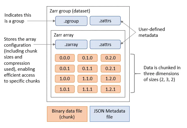
Zarr and Xarray
Xarray can open Zarr files using the open_zarr function that is similar to the open_dataset function we’ve been using to open NetCDF data. We will be using the outputs of the NEMO Near-Present-Day simulations developed by the National Oceanography Centre, specifically related to the eORCA025 model and covers the ocean globally. Each dataset can have more than 200GB, DO NOT DOWNLOAD IT!
import xarray as xr

ds = xr.open_zarr("https://noc-msm-o.s3-ext.jc.rl.ac.uk/npd-eorca025-jra55v1/T1m/so_abs")
ds
We can now see the metadata for the Zarr file. It includes 75 depth levels, 577 time steps and a 1206x1440
spatial resolution. In this case, there is only one variable, so_abs, which is the absolute salinity of the ocean. To access other variables, you can take a look on the NOC Near-Present-Day documentation. For example:
import xarray as xr

ds = xr.open_zarr("https://noc-msm-o.s3-ext.jc.rl.ac.uk/npd-eorca025-jra55v1/T1m/zos")
ds
In this case, the variable is zos, which is the “Sea Surface Height Above Geoid”. It only covers the ocean surface and don’t use the depth dimension. All of this information has come from the header of the Zarr file,
so far none of the actual data has been transferred, we have done what is known as a “lazy load” where data will only be transferred from the object store when we actually access it.
Let’s try and read it by slicing out a small part of the file, we’ll only get the zos dataset:
ssh = ds['zos'].isel(time_counter=slice(0,1),y=slice(500,700), x=slice(1000,1200))
ssh
We can see that ssh is now a 200x200x1 array that only takes up 156.25kB from the original 3.73GB file. Even at this point no data will have been transferred.
If we explore further and print the ssh array we’ll see that it is actually using a Dask array underneath.
print(ssh)
To convert this into a standard Xarray DataArray we can call .compute on the ssh.
ssh_local = ssh.compute()
We can now plot this by using:
ssh_local.plot()
Or access some of the data:
ssh_local[0,0,0]
It is important to note that this data is not on a regular grid. Therefore, slicing the data using isel will not give you an exact rectangular area, but only the data that lies within the boundaries of the grid. If you want to get a specific area, you may need to reproject the data to a regular grid. There are python libraries like iris and xESMF that help with this activity,
Plot Sea Surface Temperature
Extract and plot the sea surface temperature (
tos_convariable from thehttps://noc-msm-o.s3-ext.jc.rl.ac.uk/npd-eorca025-jra55v1/T1m/tos_confile) for the nearest date to January 1st 1965 that is in the dataset.Solution 1
import xarray as xr
ds = xr.open_zarr("https://noc-msm-o.s3-ext.jc.rl.ac.uk/npd-eorca025-jra55v1/T1m/tos_con")
sst = ds['tos_con'].sel(time_counter="1965-01-01",method="nearest")
sst.plot()
Solution 2: (OPTIONAL) plotting with Cartopy
import xarray as xr
import matplotlib.pyplot as plt
import cartopy.crs as ccrs
import cartopy.feature as cfeature
ds = xr.open_zarr("https://noc-msm-o.s3-ext.jc.rl.ac.uk/npd-eorca025-jra55v1/T1m/tos_con")
sst = ds['tos_con'].sel(time_counter="1965-01-01",method="nearest")

plt.figure(figsize=(12, 6))
ax = plt.axes(projection=ccrs.PlateCarree())

# Add white land background
ax.add_feature(cfeature.LAND, facecolor='white', zorder=1)

ax.coastlines()
pcm = ax.pcolormesh(
    sst.nav_lon, sst.nav_lat, sst,
    transform=ccrs.PlateCarree(),
    cmap="viridis",
    shading="auto",
    zorder=0  # Ensure it overlays the land
)

plt.title("Sea Surface Temperature with White Land")
plt.colorbar(pcm, label=sst.attrs.get("units", ""))
plt.tight_layout()
plt.show()
Solution 3: (OPTIONAL) reprojecting and plotting with Cartopy
# you will need to install xESMF to run this solution
# conda install -c conda-forge "esmpy=8.6.1" "esmf=8.6.1"
import xesmf as xe
import xarray as xr
import matplotlib.pyplot as plt
import cartopy.crs as ccrs
ds = xr.open_zarr("https://noc-msm-o.s3-ext.jc.rl.ac.uk/npd-eorca025-jra55v1/T1m/tos_con")
sst = ds['tos_con'].sel(time_counter="1965-01-01",method="nearest")
sst = sst.rename({'nav_lon': 'lon', 'nav_lat': 'lat'})
# Create source and target grids
ds = sst.to_dataset(name="tos_con")
# Define target regular grid (e.g., 1°)
import numpy as np
lon_target = np.linspace(-180, 180, 360)
lat_target = np.linspace(-90, 90, 180)
target_grid = xr.Dataset({
    "lon": (["lon"], lon_target),
    "lat": (["lat"], lat_target),
})
# Regrid
regridder = xe.Regridder(ds, target_grid, method="bilinear", periodic=True)
tos_regridded = regridder(ds)["tos_con"]

# Plotting the regridded data
plt.figure(figsize=(12, 6))
ax = plt.axes(projection=ccrs.PlateCarree())
pcm = ax.pcolormesh(
    tos_regridded["lon"], tos_regridded["lat"],
    tos_regridded, transform=ccrs.PlateCarree(),
    cmap="viridis"
)
ax.coastlines()
plt.title("Regridded Sea Surface Temperature")
plt.colorbar(pcm, label=sst.attrs.get("units", ""))
plt.tight_layout()
Calculate the mean sea surface temperature for two years
Calculate the mean sea surface temperature for the years between 1990 and 1991 using the same dataset as above.
Solution
import xarray as xr
ds = xr.open_zarr("https://noc-msm-o.s3-ext.jc.rl.ac.uk/npd-eorca025-jra55v1/T1m/tos_con")
sst = ds['tos_con'].sel(time_counter=slice("1990", "1991"))
grouped_mean = sst.groupby("time_counter.year").mean()
mean_sst = grouped_mean.mean(dim=['y','x']) # this will take the mean across the specified dimensions
mean_sst = mean_sst.compute()
mean_sst
Calculate the mean sea surface temperature for 10 years with Dask
Calculate the mean sea surface temperature for 1990 and 1999. Use the JASMIN Dask gateway to parallelise the calculation, use 10 worker threads and set the time_counter chunk size to 10 when opening the zarr file. Measure how long it takes to compute the result, try changing the number of workers up and down to see what the optimal number is.
Solution
import xarray as xr
import dask_gateway

gw = dask_gateway.Gateway("https://dask-gateway.jasmin.ac.uk", auth="jupyterhub")

options = gw.cluster_options()
options.worker_cores = 1
options.scheduler_cores = 1
options.worker_setup='source /apps/jasmin/jaspy/miniforge_envs/jaspy3.11/mf3-23.11.0-0/bin/activate ~/.conda/envs/esces'

clusters = gw.list_clusters()
if not clusters:
    cluster = gw.new_cluster(options, shutdown_on_close=False)
else:
    cluster = gw.connect(clusters[0].name)

client = cluster.get_client()
cluster.adapt(minimum=1, maximum=10)
client

ds = xr.open_zarr("https://noc-msm-o.s3-ext.jc.rl.ac.uk/npd-eorca025-jra55v1/T1m/tos_con")
sst = ds['tos_con'].sel(time_counter=slice("1990","1999"))
# mean_sst = dataset.mean(dim=['lat','lon']) #better way to do this
grouped_mean = sst.groupby("time_counter.year").mean()
mean_sst = grouped_mean.mean(dim=['y','x'])
result = client.compute(mean_sst).result()
result.plot()
cluster.shutdown()
Optimal workers is probably 10 and execution should take around 22 seconds. Single threaded execution time is 57 seconds.
Data Catalogues
It is a common problem that environmental scientists will need to work with datasets that span across many files. There is a common practice with larger datasets stored in Zarr or NetCDF formats to split them into multiple files with either one variable per file or one time period per file. Once we have more than a few files in our dataset keeping the correct filenames or URLs can become more difficult, especially if those names change or data gets relocated.
There are several ways to solve this problem, most of then related on building a catalogue of the dataset. This catalogue can be a simple text file that lists the filenames and URLs of the files in the dataset (like this example), or it can be a more complex database or catalogue that stores metadata about the files and their contents.
Two most used catalogues for this type of data are STAC and Intake. STAC is a standard for describing geospatial data in a way that allows it to be easily discovered and accessed, while Intake is a Python library that provides a way to manage and access datasets in a more flexible way. We will show an example using intake.
To open a catalogue we call the open_catalog function in the intake library. By converting the response of this to a Python list we can find the names of all of the datasets
in the catalogue.
import intake
xcat = intake.open_catalog('https://raw.githubusercontent.com/intake/intake-xarray/master/examples/catalog.yml')
list(xcat)
Let’s open the image example and use the skimage library to plot it
import matplotlib.pyplot as plt
image = xcat.image.read()
plt.imshow(image)
Key Points
We can process faster in parallel if we can read or write data in parallel too
Data storage is many times slower than accessing our computer’s memory
Object stores are one way to store data that is accessible over the web/http, allows replication of data and can scale to very large quantities of data.
Zarr is an object store friendly file format intended for storing large array data.
Zarr files are stored in chunks and software such as Xarray can just read the chunks that it needs instead of the whole file.
Xarray can be used to read in Zarr files
Coffee Break
Overview
Teaching: min
Exercises: minQuestions
Objectives
Feedback
In the etherpad, answer the following questions:
- Are we going too fast, too slow or just write? Record your answer in the etherpad
- What’s the most useful thing we’ve covered so far?
- What don’t you understand or would like clarification on?
Take a break!
- Drink something
- Eat something
- Talk to each other
- Get some fresh air
Key Points
GPUs
Overview
Teaching: 35 min
Exercises: 25 minQuestions
What are GPUs and how do we access them?
How can we use a GPU with Numba?
How can we use a GPU in Pandas, Numpy or SciKit Learn?
Objectives
Understand what the difference between a GPU and CPU is and the performance implications
Apply Numba to use a GPU
Understand that there are GPU enabled replacements for many popular Python libraries
Recall that NVIDIA GPUs can be programmed in CUDA, but this is a very low level operation
What are GPUs and why should we use them?
- GPUs are Graphics Processing Units, they have large numbers (100s to 1000s) of very simple processing cores and are suited to some parallel tasks like machine learning and array operations.#
- GPUs have their own RAM (memory) which their processing units can access very quickly. Any data you wish to work on must be copied from the computer (known as the “host”) to the GPU memory and any results must be copied back.
- GPUs used to have to be programmed using specialised languages/libraries such as Cuda (NVIDIA proprietary) or OpenCL (cross platform and open source).
- These are very low level systems that require the programmer to worry about things like moving data to/from GPU memory.
- Today many higher level libraries can use GPUs reducing our need to learn Cuda or OpenCL.
- For some classes of problems GPUs can give speed improvements that are 10s to hundreds of times faster than a CPU.
How can you access a GPU if your PC doesn’t have one
Many laptops and desktops won’t have very powerful GPUs, instead we’ll want to use HPC or Cloud systems to access a GPU. If you don’t have access to any services which offer one then you can use Google Colab (https://colab.research.google.com). This offers a Jupyter notebook interface with GPUs for free, but the GPUs aren’t very powerful. You can also pay for Google Colab and get access to faster GPUs.
Orchid
JASMIN has a cluster called Orchid which has 16 nodes with 72 NVIDIA A100 GPUs between them. These are accessed via the Slurm batch scheduler. For more experimental work there are some A100 GPUs attached to the JASMIN notebook service. To use these you must be granted access to Orchid and select the GPU option when connecting.
Checking what GPUs are available to us
Systems with NVIDIA GPUs usually have a command called nvidia-smi installed, this will tell us some information about the GPUs that are attached to the system.
We can invoke this either from a Jupyter terminal or in a notebook with the ! prefix.
nvidia-smi
On the JASMIN notebooks service this will return something similar to this.
+-----------------------------------------------------------------------------------------+
| NVIDIA-SMI 550.163.01             Driver Version: 550.163.01     CUDA Version: 12.4     |
|-----------------------------------------+------------------------+----------------------+
| GPU  Name                 Persistence-M | Bus-Id          Disp.A | Volatile Uncorr. ECC |
| Fan  Temp   Perf          Pwr:Usage/Cap |           Memory-Usage | GPU-Util  Compute M. |
|                                         |                        |               MIG M. |
|=========================================+========================+======================|
|   0  NVIDIA A100-SXM4-40GB          Off |   00000000:41:00.0 Off |                   On |
| N/A   34C    P0             88W /  400W |                  N/A   |     N/A      Default |
|                                         |                        |              Enabled |
+-----------------------------------------+------------------------+----------------------+
|   1  NVIDIA A100-SXM4-40GB          Off |   00000000:C1:00.0 Off |                   On |
| N/A   30C    P0             85W /  400W |                  N/A   |     N/A      Default |
|                                         |                        |              Enabled |
+-----------------------------------------+------------------------+----------------------+

+-----------------------------------------------------------------------------------------+
| MIG devices:                                                                            |
+------------------+----------------------------------+-----------+-----------------------+
| GPU  GI  CI  MIG |                     Memory-Usage |        Vol|      Shared           |
|      ID  ID  Dev |                       BAR1-Usage | SM     Unc| CE ENC DEC OFA JPG    |
|                  |                                  |        ECC|                       |
|==================+==================================+===========+=======================|
|  0    5   0   0  |              13MiB /  9856MiB    | 14      0 |  1   0    1    0    0 |
|                  |                 0MiB / 16383MiB  |           |                       |
+------------------+----------------------------------+-----------+-----------------------+
|  1    5   0   0  |              13MiB /  9856MiB    | 14      0 |  1   0    1    0    0 |
|                  |                 0MiB / 16383MiB  |           |                       |
+------------------+----------------------------------+-----------+-----------------------+

+-----------------------------------------------------------------------------------------+
| Processes:                                                                              |
|  GPU   GI   CI        PID   Type   Process name                              GPU Memory |
|        ID   ID                                                               Usage      |
|=========================================================================================|
|  No running processes found                                                             |
+-----------------------------------------------------------------------------------------+
There are two keys parts to the output here. The top part show’s we have two NVIDIA A100 cards with 40GB of GPU RAM each. However we don’t have exclusive use of these and they have been partitioned into smaller virtual GPUs known as MIGs (multi instance GPUs). Each of these only has 16GB of GPU RAM and we’re restriucted to just 10GB of that. This is still more than most desktop GPUs and is sufficient for many tasks. Where we might need more memory we will have to move our code over to a regular Python script running on Orchid’s batch system.
Checking the GPUs available to use from Python
The numba library provides an interface to Cuda, which is NVIDIA’s low level library for GPU operations. To get a list of GPUs
we can just call cuda.detect().
from numba import cuda

cuda.detect()
Check what GPUs you have access to
Ensure that you have Cuda installed, this can installed by adding the cupy and cudatoolkit packages to your Conda/Mamba environment. Use Numba/Cuda to check what version of Cuda you have installed and what GPUs you have available.
Solution
mamba install -p ~/.conda/envs/esces cupy cudatoolkitfrom numba import cuda print(cuda.__version__) cuda.detect()
Using GPUs
GPU replacements for popular libraries
NVIDIA have drop in replacements for Pandas, Numpy and SciKit learn that are GPU accelerated. The replacemnt for NumPy and SciPy is known as CuPy.
Let’s do a calculation using NumPy.
import numpy as np
a = np.random.random(100_000_000)
result_np = np.mean(a)
Now let’s try and do the same thing with CuPy.
We’ll use the same array we just created and copy it to the GPU, CuPy’s asarray function
takes in a NumPy array and converts it to a CuPy array.
import cupy as cp
b = cp.asarray(a)
result_cp = cp.mean(b)
Let’s time how long this is taking, for the NumPy code we can use %time or %timeit.
Unfortunately %time and %timeit don’t work properly with GPUs as calling a GPU function returns immediately
and the code continues to run on the GPU. So we’ll have to take a different approach to measuring the time taken and use CuPy’s
built-in profiler which includes a function called benchmark.
timeit will automatically decide how many runs to do, but defaults to 7,
whereas benchmark needs to be told how many times to repeat with the n_repeat parameter.
from cupyx.profiler import benchmark
gpu_times = benchmark(cp.mean, (b,), n_repeat=7)
print(gpu_times)
To ensure we make a comparable run using timeit we can us it’s -n and -r options
to control how many times it runs too.
%timeit -n 1 -r 7 result_np = np.mean(a)
On the JASMIN notebook service this gives the following output for CuPy:
mean : CPU: 54.157 us +/- 3.656 (min: 50.439 / max: 61.728) us GPU-0: 2158.267 us +/- 3.639 (min: 2154.080 / max: 2165.024) us
and for NumPy:
66.2 ms ± 0 ns per loop (mean ± std. dev. of 1 run, 7 loops each)
So we have used about 2ms of GPU time (plus 54us of CPU time) to take the mean of 100,000,000 numbers on the GPU and 66ms on the CPU, so that’s a 33 fold speedup! Although we did not include the time spent copying the array to the GPU.
Measuring the time taken to copy data to the GPU memory
As previously mentioned we can’t use %timeit or %time to measure how long GPU operations take. We could use benchmark to do this, but we lose the return of the function
so this won’t actually be usable (without a subsequent call). An alternative is to record the time of the system clock before and after the asarray call, but for this
to work we must synchronize with the GPU after the asarray call to ensure it’s really finished.
import time
t0 = time.time()
b = cp.asarray(a)
cp.cuda.stream.get_current_stream().synchronize()
print(str((time.time() - t0) * 1_000_000) + "us")
On JAMSIN this is taking around 100,000us or 100ms. So we need to add this to the computation time which was just 2ms. As the CPU version only took 66ms it is actually faster to do this calculation on the CPU. But this is a very simple example where we’ve only done one very simple operation on quite a large amount of data.
Create random numbers with CuPy
So far we have created random numbers using NumPy on the CPU and copied these to the GPU. A more efficient way to do this might be to make the random numbers of the GPU. Adjust the code to use CuPy to create 1,000,000 random numbers. Use the time library (or Cupyx’s benchmark) to measure how long this takes. Is this quicker than making the random numbers on the CPU?
Solution
import cupy as cp
import time

t0 = time.time()
b = cp.random.random(100_000_000)
cp.cuda.stream.get_current_stream().synchronize()
print(str((time.time() - t0)*1_000) + "ms")

#alternative using benchmark
from cupyx.profiler import benchmark
benchmark(cp.random.random, (100_000_000,), n_repeat=7)

cp.mean(b)
Using GPUs with Numba
Numba code can be converted to run on a GPU using the @cuda.jit decorator, which is similar to the @jit decorator we saw earlier on. However there are a
few alterations that code might need first due to the way GPUs operate. Firstly the functions we use on the GPU can’t return anything, we must instead have an extra
parameter which contains an array where we will save any results.
Here is an example that is similar to the function we used the JIT with earlier on with the CPU.
@cuda.jit
def sum_arr_example(a, r):
    total = 0.0
    for i in range(a.shape[0]):
        total += a[i,i]
    r[0] = total

a = cp.arange(10_000).reshape(100,100)
result_gpu = cuda.device_array((1,), np.float64)

sum_arr_example[1, 1](a, result_gpu)

result_host = result_gpu.copy_to_host()
print(result_host)
Further Reading
This has only been a very quick introduction to GPUs, but hopefully it has shown you some of the potential they offer and some simple ways to use them.
- NVIDIA Profiling Guide - NVIDIA have a very powerful visual profiling tool which graphically shows which operations are taking the most time.
- GPU Programming Carpentries Lesson - A Carpentries lesson on GPU programming including using CuPy and Numba.
- CuPy homepage
- GPU Hardware Introduction - A short video explaining the hardware architecture of a GPU.
Key Points
GPUs are Graphics Processing Units, they have large numbers of very simple processing cores and are suited to some parallel tasks like machine learning and array operations
Many laptops and desktops won’t have very powerful GPUs, instead we’ll want to use HPC or Cloud systems to access a GPU.
Google’s Colab provides free access to GPUs with a Jupyter notebooks interface.
Numba can use GPUs with minor modifications to the code.
NVIDIA have drop in replacements for Pandas, Numpy and SciKit learn that are GPU accelerated.
For a GPU to access data it must be copied into the GPU’s memory. This can sometimes be a major bottleneck to GPU operations.