Introduction
Overview
Teaching: 20 min
Exercises: 15 minQuestions
What are some of the common computing terms that I might encounter?
How can I use Python to work with large datasets?
How do I connect to a high performance computing system to run my code?
Objectives
To understand common computing terms around using HPC and Jupyter systems.
To understand what JASMIN is and the services it provides.
To have the lesson conda environment installed and running.
To be able to launch a JupyterLab instance with the lesson’s data and code present.
To be aware of the key libraries used in this lesson (Xarray, Numba, Dask, Intake).
How do we scale Python to work with big data?
Python is an increasingly popular choice for working with big data. In enviromental sciences we often encounter data that is bigger than our computer’s memory and/or that is too big to process with our desktop or laptop computers.
What are your needs?
- In the etherpad write a sentence about what kind of data you work with and how big that data is.
- Describe the problems you have working with data that is too big for your desktop or laptop computer to handle.
- List any tools, libraries and computing systems you use or have used to overcome this.
The tools we’ll look at in this lesson
In this lesson we will look at a few tools to help you work with big data and to process your data more efficiently and by using parallel processing, these will include:
- GNU Parallel
- Numpy
- Numba
- Xarray
- Dask
- Zarr
- Intake
Jargon Busting
CPU
At the heart of every computer is the CPU or Central Processing Unit. This takes the form of a microchip and typically the CPU is the biggest microchip in the computer. The CPU can be thought of as the “brain” of the computer and is what ultimately runs all of our software and carries out any operations we perform on our data.
Core
Until around 2010 most CPUs had a single processing core and could only do one thing at a time. They gave the illusion of doing multiple things at once by rapidly switching from one task to another. A few higher end computers would have multiple CPUs and could do 2/4/8 things at once if they had 2/4/8 CPUs. Since around 2010 most CPUs have multiple cores, which is effectively putting multiple CPUs onto a single chip. By having multiple cores modern computers can perform multiple tasks simultaneously.
Node/Cluster
A single computer in a group of computers known as a cluster is often called a “node”. A cluster allows us to run large programs over multiple computers with data being exchanged over a high speed network called an interconnect.
Process
A process is a single running copy of a computer program. If for example launch a (simple) Python program then it will create one Python process to run this. We can see a list of
processes running on a Linux computer with the ps or top command or on windows using the Task Manager. The computer’s operating system will decide which core should run which process
and will rapidly switch between all the running processes to ensure that they all have a chance to do some work. If a process is waiting on input from the user or for data to arrive
from a hardware device such as a disk or network then it might give up its turn to do any work until the input/data arrives. The operating system isolates each process from the others,
each will have its own memory allocated and won’t be able to read or write data to another process’s memory.
Thread
A thread is a way of having multiple things happening simultaneously inside one process. Unlike processes, threads can access each other’s memory. In multicore systems each thread might run on a different core. Some CPUs also have a feature called Hyper Threading where for every core they have some additional parts of a core, this can help run some multithreaded applications a little bit faster while only requiring a small amount of extra ciricuitry in the CPU. Some programs which tell us about the specifications of a CPU will mention how many threads a CPU has, in Hyper Threaded systems this will be double the number of cores, in non-Hyper Threaded systems it will be the same as the number of cores.
Parallel Processing
Parallel Processing is where a task is split across multiple processing cores to run different parts of it simultaneously and make it go faster. This can be acheived by using multiple processes and/or multiple threads. Bigger and more complex tasks might also be split across several computers.
Computer memory
There are two main types of computer memory, RAM or volatile storage and disk or non-volatile storage.
RAM
RAM or Random Access Memory is the computer’s short term memory, any program which is running must be loaded into RAM as is any data which that program needs. When the computer is switched off the contents of the RAM are lost. RAM is very fast to access and the “Random” in the name means it be both read from and written to. A typical modern computer might have a few gigabytes (a few billion characters) worth of RAM.
Storage
Disk or storage or non-volatile storage is where computers store things for longer term keeping. Traditionally this was on a hard disk that had spinning platters which could be magnetised (or before that on removable floppy disks which also magnetise a spinning disk). Many modern computers use Solid State Disks (SSDs) which are faster and smaller than hard disks, but they are still slower than RAM and are often more expensive. A typical modern computer might have a few hundred gigabytes to a few terabytes (trillion characters) worth of disk.
HPC systems will often have very large arrays of many disks attached to them with hundreds of terabytes or even petabytes (1000 TB) between them. On some systems this will include a mix of slower hard disks and faster but less plentiful SSDs. Some systems also have tape storage which can hold large amounts of data but is very slow to access and is typically used for backup or archiving.
Server
A server is a computer connected to a network (possibly including the internet) that accepts connections from client computers and provides them access to some kind of service, sends them some data or receives some data from them. Typically server computers have a large number of CPU cores, disk storage and/or RAM.
High Performance Computing
High Performance Computing (sometimes called Super Computing) refers to large computing systems and clusters that are typically made up of many individual computers with a large number of cores between them. They’re often used for research problems such as processing large environmental datasets or running large models and simulations such as climate models. High Performance Computing (HPC) systems are usually shared between many users. To ensure that one user doesn’t take all the resources for themselves or prevent another users program from running users are required to write a job description which tells the HPC what program they want to run and what resources it will need. This is then placed in a queue and will be run when the required resources are available. Typically when a job runs it will have a set of CPU cores dedicated to it and no other programs (apart from the operating system) will be able to use those cores.
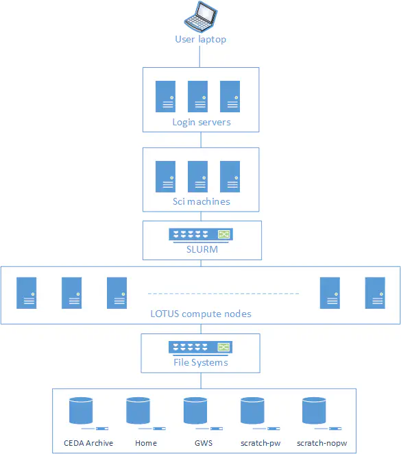
JASMIN
https://jasmin.ac.uk is the UK’s data analysis facility for data intensive environmental science. It combines several computing services together including:
- High Performance Computing system called Lotus with over 19,000 processing cores and 300 nodes.
- Virtual machines
- Jupyter Notebooks service
- Data Storage on both disk and tape
- Moderate sized shared “sci” servers, with between 8 and 48 CPU cores and 32G to 1TB of RAM
SSH
SSH or Secure SHell is a program for connecting to and running commands on another computer over a local network or the internet. As the “secure” part of the name implies, SSH encrypts all the data that it sends so that anybody intercepting the data won’t be able to read it. SSH is used to support accessing the command line interface of another computer, but it can also “tunnel” other data through the SSH connection and this can include the output of graphical programs, allowing us to run graphical programs on a remote computer.
SSH has two accompanying utilities for copying files, called SCP (Secure Copy) and SFTP (Secure File Transfer Protocol) that allow us to use SSH to copy files to or from a remote computer.
Jupyter Notebooks
Jupyter Notebooks are an interactive way to run Python (and Julia or R) in the web browser. Jupyter Lab is the program which runs a Jupyter server that we can connect to. We can run Jupyter Lab on our own computer by downloading Anaconda and running Jupyter Lab via the Anaconda Navigator, when run in this way any Python code written in the Notebook will run on our own computer. We can also use a service called a Jupyter Hub run by somebody else, usually on a server computer. When run in this way any code written in the Notebook will run on the server. This means we can take advantage of the server having more memory, CPU cores, storage or large datasets that aren’t on our computer.
Jupyter Lab also allows us to open a terminal and type in commands that run either on our computer or the Jupyter server. This can be helpful alternative to using SSH to connect to a remote server as it requires no SSH client software to be installed.
Connecting to a JupyterLab/notebooks service
We will be using the Notebooks service on the JASMIN system for this workshop. This will open a Jupyter notebook in your web browser, from this you can type in Python code and it will run on the JASMIN system. JASMIN is the UK’s data analysis facility for environmental science and co-locates both data storage and data processing facilities. It will also be possible to run much of the code in this workshop on your own computer, but some of the larger examples will probably exceed the memory and processing power of your computer.
Launching JupyterLab
In your browser connect to https://notebooks.jasmin.ac.uk. If you have an existing JASMIN account then login with your normal username and password. There is a two factor authentication on the notebook service that will email you a code, enter this code and you will be connected to the Notebook service. If you do not have a JASMIN account then please use one of the training accounts provided.
Download examples and set up the Mamba environment
To ensure we have all the packages needed for this workshop we’ll need to create a new mamba environment (mamba is a conda compatible package manger but is much faster than conda). This is defined by a YAML file that is downloaded alongside the course materials.
Download the course material
Open a terminal and type:
curl https://raw.githubusercontent.com/NOC-OI/python-advanced-esces/gh-pages/data/data.tgz > data.tgz
tar xvf data.tgz
Setting up/choosing a Mamba environment
From the terminal run the following:
curl https://raw.githubusercontent.com/NOC-OI/python-advanced-esces/refs/heads/gh-pages/data/esces-env.yml > esces-env.yml
mamba env create -f esces-env.yml -p ~/.conda/envs/esces
mamba run -p ~/.conda/envs/esces python -m ipykernel install --user --name ESCES
After about one minute if you click on the blue plus icon near the top left or the file menu and “New Launcher” option you should see a notebook option called ESCES. This will use the Mamba environment we just created and will have access to all the packages we need.
Testing package installations
Testing your package installs
Run the following code to check that you can import all the packages we’ll be using and that they are the correct versions. The !parallel runs the parallel command from the command line from within a Jupyter notebook cell. This will not work if you use stanard Python.
import xarray
import dask
import numba
import numpy
import cartopy
import intake
import zarr
import netCDF4
print("Xarray version:", xarray.__version__)
print("Dask version:", dask.__version__)
print("Numpy version:", numpy.__version__)
print("Numba version:", numba.__version__)
print("Cartopy version:", cartopy.__version__)
print("Intake version:", intake.__version__)
print("Zarr version:", zarr.__version__)
print("netCDF4 version:", netCDF4.__version__)
!parallel --version
Solution
You should see version numbers that are equal or greater than the following:
Xarray version: 2024.2.0
Dask version: 2024.3.1
Numpy version: 1.26.4
Numba version: 0.59.0
Cartopy version: 0.22.0
Intake version: 2.0.4
Zarr version: 2.17.1
netCDF4 version: 1.6.5
GNU parallel 20230522
Copyright (C) 2007-2023 Ole Tange, http://ole.tange.dk and Free Software
Foundation, Inc.
License GPLv3+: GNU GPL version 3 or later <https://gnu.org/licenses/gpl.html>
This is free software: you are free to change and redistribute it.
GNU parallel comes with no warranty.

Web site: https://www.gnu.org/software/parallel

When using programs that use GNU Parallel to process data for publication
please cite as described in 'parallel --citation'.
About the example data
There is a small example dataset included in the download above. This is a Surface Temperature Analysis from the Goddard Institute for Space Studies at NASA. It contains a monthly surface temperatures on a 2x2 degree grid from across the earth from 1880 to 2023. The data is stored in a NetCDF file. We will be using a subset of the data that runs from 2000 to 2023.
About NetCDF files
NetCDF files are suited for storing array data
They are:
- Self Describing, there is a metadata describing the whole dataset, the variables within it and their units.
- Widely supported, there are libraries to read netCDF in most programming languages and lots of tools to manipulate them.
- Python has a NetCDF4 library that can work with them, the Xarray library also works with NetCDF.
- Efficient, can store data in binary formats instead of ASCII data as CSV would.
- Able to contain multiple variables
- Contains three types of data:
- Variables: the actual data.
- Dimensions: the dimensions on which the variables exist, for example latitude, longitude and time.
- Attributes: Information about the dataset, for example who created it and when.
Exploring the GISS Temp Dataset
Load and get an overview of the dataset
import netCDF4
dataset = netCDF4.Dataset("gistemp1200-21c.nc")
print(dataset)
<class 'netCDF4.Dataset'>
root group (NETCDF4 data model, file format HDF5):
    title: GISTEMP Surface Temperature Analysis
    institution: NASA Goddard Institute for Space Studies
    source: http://data.giss.nasa.gov/gistemp/
    Conventions: CF-1.6
    history: Created 2024-03-08 11:37:27 by SBBX_to_nc 2.0 - ILAND=1200, IOCEAN=NCDC/ER5, Base: 1951-1980
    dimensions(sizes): lat(90), lon(180), time(288), nv(2)
    variables(dimensions): float32 lat(lat), float32 lon(lon), int32 time(time), int32 time_bnds(time, nv), int16 tempanomaly(time, lat, lon)
    groups:
Get the list of attributes
dataset.ncattrs()
['title', 'institution', 'source', 'Conventions', 'history']
print(dataset.title)
'GISTEMP Surface Temperature Analysis'
Get the list of variables
print(dataset.variables)
Get the list of dimensions
print(dataset.dimensions)
Read some data from out dataset
The dataset values can be read from dataset.variables['variablename'], it will have a subarray that contains the data following the dimensions specified.
In our dataset we can see that the tempanomaly variable has the shape int16 tempanomaly(time, lat, lon).
This means that time will be the first index, latitude the second and longitude the third. We can get the first timestep for the upper left coordinate by using:
print(dataset.variables['tempanomaly'][0,0,0])
One thing to note here is that our dataset’s y coordinates are backwards to most maps (following a computer graphics convention where 0 is the upper left coordinate, not the lower left or centre).
Therefore requesting [0,0,0] means the southern most and western most coordinate at the first timestep.
Read some NetCDF data
Challenge
There are 90 elements to the latitude dimension, one every two degrees and 180 in the longitude dimension, also with one every two degrees. To translate from a real latitude and longitude to an index we’ll need to divide the longitude by two and add 90 to the longitude. For the latitude we’ll need to divide by two and add 45. In Python this can be expressed as the following, we’ll also want to ensure the result is an integer by wrapping the whole calculation in
int():latitude_index = int(((latitude) / 2) + 45) longitude_index = int((longitude / 2) + 90)For the time dimension, each element represents one month starting from January 2000, so for example element 12 will be January 2001 (0-11 are January to December 2000). For example 52 degrees north (latitude) and 2 degrees west will translate to the array index 71, 91. Write some code to get the temperature anomaly for January 2020 in Astana, Kazakhstan (approximately 51 North, 71 East)
Solution
latitude = 71
longitude = 51
latitude_index = int(((latitude) / 2) + 45)
longitude_index = int((longitude / 2) + 90)
time_index = 20 * 12   #we want jan 2020, dataset starts at jan 2000 and has monthly entries
print(dataset.variables['tempanomaly'][time_index,latitude_index,longitude_index])
6.8999996
Key Points
Jupyter Lab is a system for interactive notebooks that can run Python code, these can be either on own computer or a remote computer.
Python can scale to using large datasets with the Xarray library.
Python can parallelise computation with Dask or Numba.
NetCDF format is useful for large data structures as it is self-documenting and handles multiple dimensions.
Zarr format is useful for cloud storage as it chunks data so we don’t need to transfer the whole file.
Intake catalogues make dealing with multifile datasets easier.