Converting Traditional Formats to Zarr

Estimated time: 70 minutes

Overview

Questions

• “Why convert NetCDF data to Zarr, and what changes in the way we access and process data?”
• “How do we choose chunk sizes for Zarr when starting from NetCDF files?”
• “How can we use Dask and xarray to convert and write data to Zarr efficiently?”
• “How do we test that the converted data is usable and correct (e.g. computing mean values)?”

Objectives

• “Explain the main steps in converting NetCDF datasets to Zarr.”
• “Choose appropriate chunking strategies for the target Zarr dataset.”
• “Use xarray, Dask, and to_zarr to convert NetCDF to Zarr in parallel.”
• “Upload Zarr stores to object storage and verify basic analyses on the converted data.”

Why convert NetCDF to Zarr?

---

NetCDF is widely used for ocean, climate, and meteorological data and works well on local filesystems and HPC storage. However, as datasets grow and we move to cloud and parallel computing, Zarr offers several advantages:

• Chunked storage aligned with object stores and HTTP/S3 access.
• Easy parallel reads/writes of chunks by Dask or other frameworks.
• Flexible layout for large collections (many NetCDF files → one Zarr dataset).

Converting NetCDF to Zarr does not change the scientific content, but it changes how data is organised and accessed, enabling cloud-native workflows and more efficient analysis at scale.

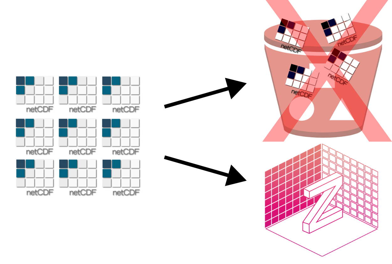
Converting from NetCDF to Zarr with xarray

To convert NetCDF to Zarr, we typically use xarray’s to_zarr method, optionally with Dask for parallelism. The following example uses the data/era5_sst/ocean_temperature.nc dataset:

1. Open data netCDF dataset with xarray:

PYTHON

import xarray as xr
base_path = "/gws/ssde/j25b/atlantis_vis/cloud-native-geoscience-course/" # or "" if you have the data in your current working directory
ds_nc = xr.open_dataset(f"{base_path}data/era5_sst/ocean_temperature.nc")
print(ds_nc)

2. Decide how the dataset should be chunked

The chunking scheme should match the way the data will be used later. A simple example chunking choice might look like this:

PYTHON

ds_nc = ds_nc.chunk({"valid_time": 10, "latitude": 100, "longitude": 100})
print(ds_nc.chunks)

3. Write the Zarr store

Once the chunking looks right, write the dataset to Zarr.

PYTHON

ds_nc.to_zarr("data/example.zarr", mode="w")

Now you have a local Zarr store that can be uploaded to object storage and accessed in parallel by multiple clients:

PYTHON

ds_zarr = xr.open_zarr("data/example.zarr")
print(ds_zarr)

Challenge

Exercise 1 - Convert a NetCDF dataset to Zarr

Using the NetCDF dataset provided (data/era5_sst/ocean_temperature.nc), open a single file with open_dataset, chunk it with {"valid_time": 10, "latitude": 100, "longitude": 100}, and write it to a local Zarr store.

Then, reopen the Zarr store and verify that the dimensions and variables match the original NetCDF dataset, and if the chunking is as expected.

Show me the solution

PYTHON

import xarray as xr

base_path = "/gws/ssde/j25b/atlantis_vis/cloud-native-geoscience-course/" # or "" if you have the data in your current working directory

ds_nc = xr.open_dataset(f"{base_path}data/era5_sst/ocean_temperature.nc")
ds_nc = ds_nc.chunk({"valid_time": 10, "latitude": 100, "longitude": 100})
ds_nc.to_zarr("data/example.zarr", mode="w")

PYTHON

ds_zarr = xr.open_zarr("data/example.zarr")
print(ds_zarr)

Overall workflow: NetCDF → Zarr → object store

---

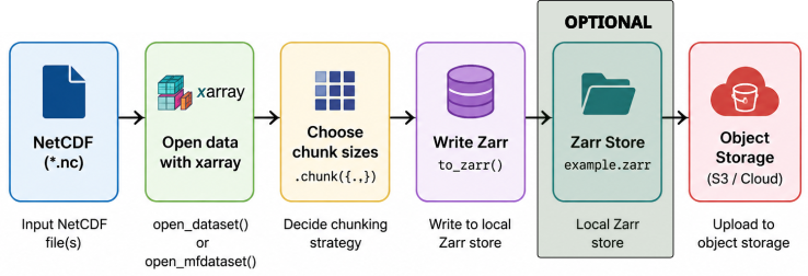
In the real world, the conversion of NetCDF to Zarr is often done in a workflow that includes the following typical steps:

1. Understand the NetCDF input: check variables, dimensions, coordinates, and chunking.
2. Decide chunking strategy for Zarr: based on expected access patterns and approximate chunk sizes in MB.
3. Open NetCDF with xarray: using open_dataset or open_mfdataset for multiple files.
4. Apply chunking and encoding: use .chunk() and define any compression or encoding options.
5. (Optional) Write Zarr to local storage: using Dataset.to_zarr(), possibly with Dask for parallel writes.
6. Upload Zarr store to object storage: using cloud CLI tools or filesystem libraries, or directly write to object storage with fsspec.
7. Verify by reopening from object storage and running analyses (e.g. computing mean values).

We’ll walk through these steps conceptually and via exercises. For the example below, we will use a subset of the GLORYS Reanalysis dataset. The data is located in the data/glorys/ directory and is provided as multiple NetCDF files, one per day. The goal is to convert this collection of NetCDF files into a single Zarr store that can be accessed efficiently in parallel.

NetCDF-to-Zarr conversion should include chunk design, validation, and publishing checkpoints.

Step 1 - Inspect NetCDF inputs

---

Before converting, inspect the NetCDF file(s) you plan to convert.

Example of opening a single NetCDF file:

PYTHON

import xarray as xr

ds_nc = xr.open_dataset(f"{base_path}data/glorys/glorys_20260501.nc")
print(ds_nc)
print(ds_nc.dims)
print(ds_nc.data_vars)
print(ds_nc.coords)
print(ds_nc.encoding)  # may show chunking and compression info

Questions to answer:

• Are there multiple files (e.g. one per time slice) or just a single file?
• Which dimensions are present (e.g. time, lat, lon, depth, member)?
• Are variables chunked already, and if so, how?
• Are all files consistent in terms of variables and coordinates if you plan to use open_mfdataset?

Because we have multiple NetCDF files, we can use open_mfdataset to open them all at once:

PYTHON

ds_nc_multi = xr.open_mfdataset(
    f"{base_path}data/glorys/*.nc",
    combine="by_coords",
)
print(ds_nc_multi)

It is important to mention that open_mfdataset will combine multiple files into a single xarray dataset, but it requires that the variables and coordinates are consistent across files. And we are not loading the data into memory yet. Xarray will lazily load data as needed.

Step 2 - Decide chunking strategy for Zarr

---

Chunks in Zarr have a major impact on performance. A common rule of thumb is to aim for compressed chunk sizes in the range of 10-100 MB, but exact choices depend on workloads and hardware.

Consider:

• Dimensions: which ones correspond to time, space, depth, ensemble member?
• Workloads: time series at points, spatial means, regional subsets, ensemble statistics.
• Storage: local HPC disk vs object store, network bandwidth, parallel framework (Dask).

Example chunk strategy for a dataset with dimensions (time, latitude, longitude, depth):

• If time series are common: {"time": 360, "latitude": 100, "longitude": 100, "depth": 1}.
• If spatial maps per time are common: {"time": 1, "latitude": 361, "longitude": 720, "depth": 1}.
• If depth slices are common: {"time": 1, "latitude": 100, "longitude": 100, "depth": 10}.

You can experiment with different chunk shapes and use Dask’s dashboard and performance measurements to refine choices.

Step 3 - Convert NetCDF to Zarr with xarray and Dask

---

Once chunking decisions are made, you can use xarray’s to_zarr method to write out the dataset. This can be done serially or in parallel using Dask. For large datasets, parallel writing is often necessary to avoid long runtimes.

First, create a Dask client to manage parallelism:

PYTHON

from dask.distributed import Client
import xarray as xr

client = Client(n_workers=2, threads_per_worker=2)

Then, open the NetCDF dataset and apply chunking:

PYTHON

ds_nc = xr.open_mfdataset(f"{base_path}data/glorys/*.nc", combine="by_coords")

# Choose chunking
ds_chunked = ds_nc.chunk({"time": 5, "latitude": 400, "longitude": 400, "depth": 10})

Now you can write the chunked dataset to Zarr. You can choose to consolidate metadata for faster reads later:

PYTHON

ds_chunked.to_zarr("data/glorys.zarr", mode="w", consolidated=True)

Open the Zarr store to verify:

PYTHON

ds_zarr = xr.open_zarr("data/glorys.zarr", consolidated=True)
print(ds_zarr)

Callout

Consolidated metadata

When writing a Zarr store, you can choose to consolidate metadata. This means the store writes a single metadata index file, that collects the metadata for all arrays and attributes in one place.

This is useful because opening the dataset can be faster, especially when the store has many variables or many chunks. Instead of reading lots of small metadata files one by one, xarray can read the consolidated metadata in a single step.

A good practice is to use consolidated metadata when the dataset will be read many times after writing, especially in cloud or object-store workflows. It is usually a good default for analysis-ready Zarr stores.

Callout

Encoding and compression

When writing Zarr stores, you can choose how each variable is encoded and compressed. In most teaching and analysis workflows, the goal is not to maximise compression at all costs, but to choose a strategy that balances file size, speed, and ease of reading.

A simple example looks like this:

PYTHON

import zarr
from zarr.codecs import BloscCodec, BloscShuffle
import xarray as xr

ds = xr.open_dataset(f"{base_path}data/era5_sst/ocean_temperature.nc")
compressor = BloscCodec(cname="zstd", clevel=3, shuffle=BloscShuffle.shuffle)
encoding = {
    "sst": {
        "compressors": compressor,
        "chunks": (10, 100, 100),
    }
}

ds.to_zarr(
    "data/example_compressed.zarr",
    mode="w",
    encoding=encoding,
    consolidated=True,
)

In this example: - zstd gives good compression with reasonable speed. - clevel=3 is a moderate compression level, which is often a good compromise between speed and size. - shuffle=2 usually improves compression for many numerical datasets. - The same compressor is applied to each data variable through the encoding dictionary.

For scientific data, moderate compression is often a good default because it reduces storage size, lower network transfer costs, and keeps read/write speeds reasonable. Very aggressive compression can save more space, but it may slow down writing and reading. For large workflows, that trade-off is often not worth it.

Step 4 - Upload Zarr to object storage

---

After successfully writing Zarr locally, you can upload the Zarr directory store to an object store (AWS S3, GCS, MinIO, etc.).

The following example uses s3cmd, which is a command-line tool for interacting with S3-compatible object stores. You can also use other tools like awscli, rclone, or Python libraries like boto3 or fsspec.

BASH

# Create a bucket (if it doesn't exist)
s3cmd mb s3://my-bucket

# Upload the Zarr store recursively
s3cmd put -r data/glorys.zarr s3://my-bucket/glorys.zarr

Once uploaded, you can access the Zarr store directly from the object store using xarray and filesystem adapters, as in previous lessons.

In our lesson here, instead of generating the zarr dataset locally and upload then later to the object store, we will directly write the zarr dataset to the object store using fsspec. This is a more efficient approach and avoids unnecessary local storage usage. In the code below, remember to replace my-bucket with the actual bucket name you have access to (please ask the instructor for the bucket name and credentials).

Because the dataset is large, we will use the JASMIN dask cluster to run the conversion and upload, as it has better network access to the object store. You can see an example below, but you can also take a look in the Parallel Processing for Zarr episode for more details.

Create a connection to dask-gateway and start a cluster:

PYTHON

import dask_gateway

# Create a connection to dask-gateway.
gw = dask_gateway.Gateway("https://dask-gateway.jasmin.ac.uk", auth="jupyterhub")

options = gw.cluster_options()
options.worker_cores = 4
options.scheduler_cores = 2
options.account = "workshop"
options.worker_setup='source /apps/jasmin/jaspy/miniforge_envs/jaspy3.11/mf3-23.11.0-0/bin/activate /work/scratch-nopw2/tobfer/cloud-native-geoscience-course'
clusters = gw.list_clusters()
if not clusters:
    cluster = gw.new_cluster(options, shutdown_on_close=False)
else:
   cluster = gw.connect(clusters[0].name)
client = cluster.get_client()
cluster.adapt(minimum=1, maximum=4)

Create a mapper for the object store:

PYTHON

import xarray as xr
import fsspec
import os

store_url = "s3://my-bucket/glorys.zarr"

# remember to set the AWS_ACCESS_KEY_ID and AWS_SECRET_ACCESS_KEY environment variables with your credentials
os.environ["AWS_ACCESS_KEY_ID"] = "your-access-key"
os.environ["AWS_SECRET_ACCESS_KEY"] = "your-secret-key"

storage_options = {
    "key": os.environ["AWS_ACCESS_KEY_ID"],
    "secret": os.environ["AWS_SECRET_ACCESS_KEY"],
    "client_kwargs": {"endpoint_url": "https://atlantis-vis-o.s3-ext.jc.rl.ac.uk"},
    # The `config_kwargs` is required for JASMIN S3 object store.
    "config_kwargs": {
        "request_checksum_calculation": "when_required",
        "response_checksum_validation": "when_required",
    },
}

# Create a mapper for the object store
mapper = fsspec.get_mapper(
    store_url,
    **storage_options,
)

Write the dataset directly to the object store:

PYTHON

ds_chunked.to_zarr(
    mapper,
    mode="w",
    consolidated=True,
)

Step 5 - Verify with a simple analysis

---

To verify that the converted Zarr dataset is usable, run a simple analysis, such as computing a mean value. Example:

PYTHON

import xarray as xr
import fsspec

# Replace `my-bucket` with the actual bucket name you have access to.
mapper = fsspec.get_mapper(
    store_url,
    **storage_options,
)
ds_zarr = xr.open_zarr(mapper, consolidated=True)

# You can also access the dataset directly, as it is in a public bucket (replace with your own bucket if needed):
ds_zarr = xr.open_zarr("https://atlantis-vis-o.s3-ext.jc.rl.ac.uk/my-bucket/glorys.zarr", consolidated=True)

# Choose a variable
var = ds_zarr["zos"]

# Mean for each time step (global spatial mean)
mean_per_time = var.mean(dim=("latitude", "longitude")).compute()
print(mean_per_time)

# Mean for each latitude/longitude location (time mean)
mean_per_latlon = var.mean(dim="time").compute()
print(mean_per_latlon)

Challenge

Exercise 2 - Understand your NetCDF dataset

For the exercises 2-5, we are going to work with the subset of the ERA5 Reanalysis dataset related to the variable swh (significant wave height). The dataset is provided as multiple NetCDF files, one per day, in the data/daily_swh/ directory.

Using the NetCDF dataset(s) provided on the server:

1. Open a single file with open_dataset and print:
   • Dimensions and coordinates.
   • Data variables.
   • Encoding information (especially chunking).
2. Then, open multiple files with open_mfdataset and verify:
   • Consistency of variables and coordinates.
   • Combined time dimension length.

What are the main variables and dimensions you care about, and what is the existing chunking layout (if any)?

Show me the solution

Open a single NetCDF file:

PYTHON

import xarray as xr
ds_nc = xr.open_dataset(f"{base_path}data/daily_swh/swh_2025-01-01.nc")
print(ds_nc.dims)
print(ds_nc.data_vars)
print(ds_nc.coords)
print(ds_nc.encoding)

Open multiple NetCDF files:

PYTHON

ds_nc = xr.open_mfdataset(
    f"{base_path}data/daily_swh/swh_*.nc",
    combine="by_coords",
)
print(ds_nc.dims)
print(ds_nc.data_vars)
print(ds_nc.coords)

Now you should have a clear picture of the input data: variables, dimensions, coordinates, and any existing chunking or compression. This understanding is essential before deciding a Zarr chunk layout or doing any conversion.

Challenge

Exercise 3 - Propose Zarr chunk sizes

Based on your NetCDF dataset and expected workloads:

1. Propose a chunk dictionary, e.g. {"time": 720, "lat": 100, "lon": 100} or similar.
2. Estimate (roughly) the size of each chunk in bytes/MB (using variable sizes and dimension lengths).
3. Explain how your chunk choices support your intended analyses.

You do not need exact numbers. Focus on reasoning.

Show me the solution

PYTHON

# Example chunk proposal
chunking = {"time": 720, "latitude": 100, "longitude": 100}

chunk_size_bytes = (
    ds_nc["swh"].dtype.itemsize  # bytes per element
    * chunking["time"]
    * chunking["latitude"]
    * chunking["longitude"]
)
chunk_size_MB = chunk_size_bytes / (1024 ** 2)
print(f"Estimated chunk size: {chunk_size_MB:.2f} MB")

After calculating the estimated chunk size, you can reason about how this chunking supports your analysis:

PYTHON

ds_chunked = ds_nc.chunk(chunking)

You’d propose reasonable chunk sizes that reflect your workloads and aim for manageable chunk sizes. You will practice linking chunk shapes to analysis patterns, preparing for actual conversion.

Challenge

Exercise 4 - Convert your NetCDF dataset to Zarr in object storage

After opening and chunking the NetCDF dataset, convert it to Zarr and write it directly to the object store using fsspec.

Please use the credentials provided by the instructor to access the object store. For this exercise, use the JASMIN Dask cluster (or the local Cluster) to perform the conversion and upload, as it provides better network access to the object store. You can refer to the Parallel Processing for Zarr episode for more details.

Once the conversion is complete, reopen the dataset from the object store and verify that it can be read correctly.

Questions:

• How long did the conversion and upload take?
• Does the size of the Zarr store seem reasonable compared to the original NetCDF files?
• Were there any variables or attributes you needed to drop or adjust?
• Does the reopened dataset have the expected dimensions, variables, and attributes?

Show me the solution

First, create a Dask cluster and connect a client. You can use a local Cluster:

PYTHON

from dask.distributed import Client

client = Client(n_workers=2, threads_per_worker=2)

Or a JASMIN Dask cluster:

PYTHON

import dask_gateway

# Create a connection to dask-gateway.
gw = dask_gateway.Gateway(
    "https://dask-gateway.jasmin.ac.uk",
    auth="jupyterhub",
)

options = gw.cluster_options()
options.worker_cores = 2
options.scheduler_cores = 1
options.account = "workshop"
options.worker_setup = (
    "source /apps/jasmin/jaspy/miniforge_envs/jaspy3.11/"
    "mf3-23.11.0-0/bin/activate "
    "/work/scratch-nopw2/tobfer/cloud-native-geoscience-course"
)

clusters = gw.list_clusters()
if not clusters:
    cluster = gw.new_cluster(options, shutdown_on_close=False)
else:
    cluster = gw.connect(clusters[0].name)

client = cluster.get_client()
cluster.adapt(minimum=1, maximum=4)

Then convert the dataset directly to object storage and reopen it:

PYTHON

import os
import xarray as xr
import fsspec

storage_options = {
    "key": os.environ["AWS_ACCESS_KEY_ID"],
    "secret": os.environ["AWS_SECRET_ACCESS_KEY"],
    "client_kwargs": {
        "endpoint_url": "https://atlantis-vis-o.s3-ext.jc.rl.ac.uk",
    },
    "config_kwargs": {
        "request_checksum_calculation": "when_required",
        "response_checksum_validation": "when_required",
    },
}

store_url = "s3://my-bucket/era5_swh.zarr"
mapper = fsspec.get_mapper(
    store_url,
    **storage_options,
)

ds_chunked.to_zarr(
    mapper,
    mode="w",
    consolidated=True,
)

ds_zarr = xr.open_zarr(
    mapper,
    consolidated=True,
)

print(ds_zarr)

Writing directly to object storage avoids creating an intermediate local copy and reflects a typical cloud-native workflow. Reopening the dataset verifies that the conversion completed successfully and that the dataset structure and metadata have been preserved.

The time taken for conversion and upload will depend on the dataset size, chunking, network speed, and cluster resources. You can use Dask’s dashboard to monitor progress and performance.

Challenge

Exercise 5 - Check consistency and compute a mean

Using both the original NetCDF files dataset (ds_nc) and the converted Zarr dataset (ds_zarr from object storage):

1. Compute the same statistic in both cases (e.g. global mean temperature at a given time):
2. Compare the results for equality (or near-equality within floating point tolerance).
3. Compare the time taken to open the dataset and compute the statistic in both cases.

Show me the solution

PYTHON

import time

# NetCDF
t0 = time.time()
ds_nc = xr.open_mfdataset(f"{base_path}data/daily_swh/swh_*.nc", combine="by_coords")
var_nc = ds_nc["swh"]
# slice to a single time step for comparison
var_nc = var_nc.isel(time=0)
t1 = time.time()
mean_nc = var_nc.mean(dim=("latitude", "longitude"))

t2 = time.time()
print("NetCDF mean:", float(mean_nc.values))
print("Time to open NetCDF files:", t1 - t0, "seconds")
print("Time taken for NetCDF computation:", t2 - t1, "seconds")
print("Total time for NetCDF:", t2 - t0, "seconds")

# Zarr
t0 = time.time()
ds_zarr = xr.open_zarr("https://atlantis-vis-o.s3-ext.jc.rl.ac.uk/my-bucket/era5_swh.zarr", consolidated=True)
var_zarr = ds_zarr["swh"]
var_zarr = var_zarr.isel(time=0)
t1 = time.time()
mean_zarr = var_zarr.mean(dim=("latitude", "longitude"))
mean_zarr = mean_zarr.compute()
t2 = time.time()
print("Zarr mean:", float(mean_zarr.values))
print("Time to open Zarr store:", t1 - t0, "seconds")
print("Time taken for Zarr computation:", t2 - t1, "seconds")
print("Total time for Zarr:", t2 - t0, "seconds")

When done carefully, converting NetCDF to Zarr and back preserves scientific values. The mean values should match within floating point tolerance, confirming that the conversion workflow is valid.

Key Points

• “Converting NetCDF to Zarr enables cloud-native, chunked, and parallel-friendly access to large scientific datasets.”
• “Effective conversion requires understanding input data, choosing chunk sizes based on workloads, and using xarray’s to_zarr with appropriate encoding and compression.”
• “Dask can parallelise the conversion process, making it feasible to handle large collections of NetCDF files.”
• “Uploading Zarr stores to object storage allows distributed teams and tools to access the same datasets efficiently.”
• “Checking basic statistics (e.g. mean values) in NetCDF and Zarr versions helps verify that conversions preserve scientific content.”