Summary and Schedule

Introduction

---

This lesson provides the preparation needed before the main Cloud-Native Architectures and Modern Data Formats for Geoscience course.

It includes three episodes:

1. Shell basics for navigating files, editing text, and using help tools.
2. Introductory xarray workflows for opening, slicing, plotting, and processing NetCDF data.
3. Git foundations for tracking changes, branching, and merging.

The goal is to ensure all learners begin the main course with a shared baseline in command-line, Python data handling (using xarray), and version control workflows.

And it also includes a setup guide for installing the required software and Python packages.

	Setup Instructions	Download files required for the lesson
Duration: 00h 00m	1. Getting Started with the Shell	“How do I install and open a shell on my computer?” “What is a shell, and why should I use it instead of only a graphical interface?” “How do I move around directories and inspect files from the command line?” “How do I do common file and folder operations in Bash?” “How can I get help when I do not remember a command?”
Duration: 00h 45m	2. Working with data in Xarray	“How do I load data with Xarray?” “How does Xarray index data?” “How do I apply operations to the whole or part of an array?” “How do I work with time series data in Xarray?” “How do I visualise data from Xarray?”
Duration: 02h 15m	3. Introduction to Git	“How do I install and configure Git on my machine?” “Why do I need a GitHub account for collaborative workflows?” “How do add, status, diff, and commit work together?” “How do I inspect what changed and when?” “How do branches help me work safely on new changes?” “How do I merge branch work back into main?”
Duration: 03h 30m	Finish

The actual schedule may vary slightly depending on the topics and exercises chosen by the instructor.

Setup

---

In the “Cloud-Native Architectures and Modern Data Formats for Geoscience course”, we will use:

• jupyterlab
• numpy
• netCDF4
• xarray
• zarr
• dask
• fsspec, s3fs, boto3, and obstore for cloud storage access
• matplotlib and cartopy for plotting
• icechunk for versioning
• virtualizarr for virtual Zarr stores
• stac for cataloging
• topozarr for multiscale Zarr visualization
• others…

The exact environment is provided in the course repository as an environment.yml file for creating a conda environment.

Accessing the workshop environment

---

There are two ways to join the workshop:

• In person: use a JASMIN training account and the JASMIN notebook service.
• Remote: download the data locally and install the environment on your own computer.

In-person setup (JASMIN)

We will be using the Notebooks service on the JASMIN system for this workshop. This will open a Jupyter notebook in your web browser, from which you can type in Python code and it will run on the JASMIN system. JASMIN is the UK’s data analysis facility for environmental science and co-locates both data storage and data processing facilities. It will also be possible to run much of the code in this workshop on your own computer, but some of the larger examples will probably exceed the memory and processing power of your computer.

You received an email with instructions to access a JASMIN training account.

Launching JupyterLab

In your browser, connect to https://notebooks.jasmin.ac.uk. Please use the username and password provided in your training account by email. There is a two-factor authentication step on the notebook service that will email you a code; enter this code and you will be connected to the Notebook service.

Setting up the environment

A preconfigured Conda environment is available for use: cloud-native-geoscience-course. This environment includes all necessary packages and dependencies and is built using the environment.yml file available here.

Since the environment is stored in a non-standard location (/work/scratch-nopw2/tobfer/cloud-native-geoscience-course-env), Jupyter will not detect it automatically. Follow these steps to set it up:

• Open a Terminal.

From the Jupyter launcher, click the Terminal icon.

• Register the cloud-native-geoscience-course kernel.

Run the following command:

BASH

mamba run -p /work/scratch-nopw2/tobfer/cloud-native-geoscience-course-env python -m ipykernel install --user --name cloud-native-geoscience-course

If the command above fails, try running these commands first, then repeat the registration step:

BASH

mamba init
exec bash

• Launch Jupyter with the cloud-native-geoscience-course environment.

Open a new Jupyter launcher by clicking File > New Launcher. Then a new notebook and console option named cloud-native-geoscience-course should now be available. This may take about a minute to appear.

Jupyter kernel choice

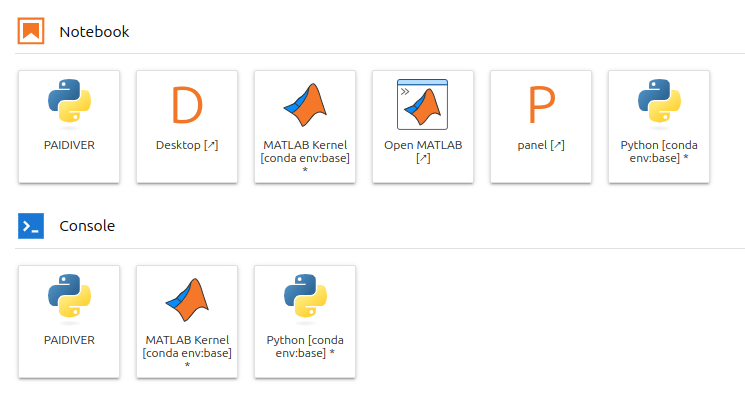
Click on cloud-native-geoscience-course to open a notebook.

Data access

In-person participants will use a shared JASMIN group workspace for the example data. You do not need to download the data locally. You only need to confirm that you can access the folder and read the files.

Please run the following command in a terminal on the JASMIN notebook service to check that you can access the data:

BASH

ls /gws/ssde/j25b/atlantis_vis/cloud-native-geoscience-course/

If you see a folder called data, you have access to the example data. If you see an error, please ask for help.

During the course, remember to use the full path /gws/ssde/j25b/atlantis_vis/cloud-native-geoscience-course/ when accessing the data.

Remote setup (your own computer)

If you are joining remotely, you will install the environment on your own computer.

Before you start

You will need:

• Python 3.13 or newer.
• Conda or mamba installed.
• Core i5 or newer CPU, with 8 cores preferred.
• At least 16 GB of RAM, with 32 GB preferred.
• At least 4 GB of free disk space for the environment.
• At least 30 GB of free disk space for the example data and for data that will be generated during the workshop.
• A stable internet connection for downloading packages and data.
• A terminal application (e.g., Terminal on macOS, Console or Terminal in Linux, or Git Bash or WSL on Windows).

Below I’ll explain the steps to install Python and conda/mamba on your own computer. If you already have a working Python 3.13 installation with conda or mamba, you can skip to the next section.

Install Miniforge

First, install Conda on your machine, if you don’t already have it. You can install the Anaconda distribution. This is a conda distribution that includes many scientific packages. If you install Anaconda, you will have a working Python environment with conda already installed.

However, Anaconda is large and may take a long time to install.

Another option is to install Miniforge for your OS. As the name suggests, Miniforge is a “mini” version of the Anaconda Python distribution that includes only Conda, a Python 3 distribution, and any necessary OS-specific dependencies.

If you already have Conda on your machine, you can skip this step.

For convenience, here are links to the 64-bit Miniforge installers:

• Windows
• Mac OSX - Intel CPU
• Mac OSX - Apple M1/2/3 CPU
• Linux

Windows installation

If you are using miniforge on Windows, after you download the Windows installer, double-click it and follow the instructions, including accepting the license.

Make sure you tick the “Add Miniforge3 to my PATH environment variable” option.

Mac OSX or Linux installation

If you are using miniforge on Mac OSX or Linux, you can install it from the command line. First, download the 64-bit Python 3 install script for Miniforge either by clicking the link above or using this command in your terminal:

BASH

wget "https://github.com/conda-forge/miniforge/releases/latest/download/Miniforge3-$(uname)-$(uname -m).sh"

Run the Miniforge install script from your terminal. Follow the prompts on the installer screens. If you are unsure about any setting, accept the defaults.

BASH

bash Miniforge3-$(uname)-$(uname -m).sh

Once the install script completes, you can remove it.

BASH

rm Miniforge3-$(uname)-$(uname -m).sh

Verifying your Conda installation

To verify that you have installed Conda correctly, run the conda --help command. The output should look similar to the following.

BASH

$ conda --help
usage: conda [-h] [-V] command ...

conda is a tool for managing and deploying applications, environments and packages.

Options:

positional arguments:
  command
    clean        Remove unused packages and caches.
    config       Modify configuration values in .condarc. This is modeled
                 after the git config command. Writes to the user .condarc
                 file (/Users/drpugh/.condarc) by default.
    create       Create a new conda environment from a list of specified
                 packages.
    help         Displays a list of available conda commands and their help
                 strings.
    info         Display information about current conda install.
    init         Initialize conda for shell interaction. [Experimental]
    install      Installs a list of packages into a specified conda
                 environment.
    list         List linked packages in a conda environment.
    package      Low-level conda package utility. (EXPERIMENTAL)
    remove       Remove a list of packages from a specified conda environment.
    uninstall    Alias for conda remove.
    run          Run an executable in a conda environment. [Experimental]
    search       Search for packages and display associated information. The
                 input is a MatchSpec, a query language for conda packages.
                 See examples below.
    update       Updates conda packages to the latest compatible version.
    upgrade      Alias for conda update.

optional arguments:
  -h, --help     Show this help message and exit.
  -V, --version  Show the conda version number and exit.

conda commands available from other packages:
  env

At the bottom of the help menu you will see a section with some optional arguments for the conda command. In particular, you can pass the --version flag, which will return the version number. Again, the output should look similar to the following:

BASH

$ conda --version
conda 24.11.3 # or similar, depending on the version you installed

Recommended folder layout

We suggest a simple folder structure like this:

cloud-native-geoscience-course/
├── environment/
└── data/

Keep the environment files in cloud-native-geoscience-course/environment/ and the data in cloud-native-geoscience-course/data/. And save all the jupyter notebooks you create in the cloud-native-geoscience-course/ folder. This will make it easier to find your files later.

Please create the cloud-native-geoscience-course/ folder in your home directory, and then create the environment/ and data/ subfolders.

BASH

mkdir -p ~/cloud-native-geoscience-course/environment
mkdir -p ~/cloud-native-geoscience-course/data

Install the environment

Download the environment.yml file from the lesson repository:

BASH

cd ~/cloud-native-geoscience-course/environment

curl -L https://raw.githubusercontent.com/NOC-OI/prep-work-cloud-native-geoscience-course/refs/heads/main/episodes/files/environment.yml -o environment.yml

Then create the environment:

BASH

conda env create -f environment.yml

Note1: This command can take several minutes to complete, depending on your internet connection and computer speed.

Note2: For Windows users that are using git bash, they reported problems with the library tree inside the environment.yml file. If you had problems with this library while creating the environment, try removing it from the environment.yml file and then create the environment again.

This will create a new environment with all the required packages. The environment name is defined in the environment.yml file, and it is cloud-native-geoscience-course for this workshop. Now activate the environment:

BASH

conda activate cloud-native-geoscience-course

If the command above fails, try running these commands first, then repeat the activation step:

BASH

conda init
exec bash

Download the example data

Remote participants need to download the example data locally.

The full example data is about 20 GB, so make sure you have enough free disk space before you start.

Download the zip file from the lesson repository, then unzip it into your cloud-native-geoscience-course/data/ folder:

BASH

curl -L https://atlantis-vis-o.s3-ext.jc.rl.ac.uk/cloud-native-geoscience-course/cloud-native-geoscience-course-data.tar.gz -o ~/cloud-native-geoscience-course/data.tar.gz
tar -v -xzf ~/cloud-native-geoscience-course/data.tar.gz -C ~/cloud-native-geoscience-course/

Note: The extraction process can take some time, because we are extracting a large number of files. After the process completes, you can check if the daily_swh, era5_sst, and glorys folders were created inside data folder by running ls -lh ~/cloud-native-geoscience-course/data/.

If you already have the three folders mentioned above, you can delete the original compressed file to free up space on your computer.

BASH

rm ~/cloud-native-geoscience-course/data.tar.gz

Launch Python interface

To start working with Python, we need to launch a program that will interpret and execute our Python commands. In this workshop, we are working mainly in Jupyter notebooks.

A Jupyter notebook provides a browser-based interface for working with Python. You can launch a notebook from the terminal:

Unix shell

Navigate to the cloud-native-geoscience-course/ directory. If you’re using a Unix shell application, such as Terminal on macOS, Console or Terminal in Linux, or [Git Bash][gitbash] on Windows, execute the following command:

BASH

cd ~/cloud-native-geoscience-course/

To launch the Jupyter server, run:

BASH

jupyter lab

Command Prompt (Windows)

On Windows, you can use its native Command Prompt program. The easiest way to start it up is by pressing Windows Logo Key+R, entering cmd, and hitting Return. In the Command Prompt, use the following command to navigate to the cloud-native-geoscience-course/ folder:

cd /D %userprofile%\cloud-native-geoscience-course/

To launch the Jupyter server, run:

python -m jupyter lab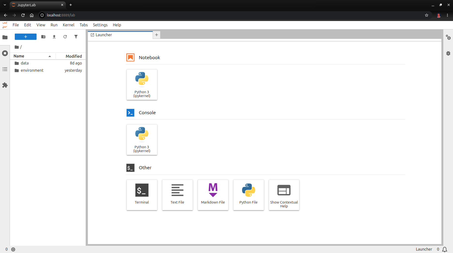

Access the notebooks

Once the Jupyter server is running, it will open a new tab in your web browser showing the notebook dashboard. Launch the notebook by clicking on the “Python 3 (ipykernel)” button on the “Notebook” session, not in the “Console” or “Other”:

Test the installation

Run the following code to check that the core packages are available:

PYTHON

import numpy
import pandas
import xarray
import s3fs
import dask
import dask_gateway
import zarr
import netCDF4
import matplotlib
import cartopy
import fsspec
import icechunk
import virtualizarr
import pystac
import topozarr
import boto3
import shapely
import obstore
import eccodes
import cfgrib
import OceanDataStore

print("numpy:", numpy.__version__)
print("pandas:", pandas.__version__)
print("xarray:", xarray.__version__)
print("s3fs:", s3fs.__version__)
print("dask:", dask.__version__)
print("dask_gateway:", dask_gateway.__version__)
print("zarr:", zarr.__version__)
print("netCDF4:", netCDF4.__version__)
print("matplotlib:", matplotlib.__version__)
print("cartopy:", cartopy.__version__)
print("fsspec:", fsspec.__version__)
print("icechunk:", icechunk.__version__)
print("virtualizarr:", virtualizarr.__version__)
print("pystac:", pystac.__version__)
print("topozarr:", topozarr.__version__)
print("boto3:", boto3.__version__)
print("shapely:", shapely.__version__)
print("obstore:", obstore.__version__)
print("eccodes:", eccodes.__version__)
print("cfgrib:", cfgrib.__version__)
print("OceanDataStore:", OceanDataStore.__version__)

You should see something like:

OUTPUT

numpy: 2.4.3
pandas: 3.0.2
xarray: 2026.7.0
s3fs: 2026.4.0
dask: 2026.3.0
dask_gateway: 2026.3.0
zarr: 3.2.1
netCDF4: 1.7.4
matplotlib: 3.11.1
cartopy: 0.25.0
fsspec: 2026.4.0
icechunk: 2.1.1
virtualizarr: 2.7.1
pystac: 1.15.2
topozarr: 0.1.2
boto3: 1.43.46
shapely: 2.1.2
obstore: 0.11.0
eccodes: 2.48.0
cfgrib: 0.9.15.1
OceanDataStore: 0.3.0

About the example data

---

The “Cloud-Native Architectures and Modern Data Formats for Geoscience” course uses example ocean and atmospheric datasets in NetCDF, GRIB, and Zarr formats to demonstrate different approaches for storing and accessing scientific data.

The datasets are derived from widely used public products, including:

• ERA5 hourly data on single levels from the Copernicus Climate Data Store (ECMWF). ERA5 is the fifth-generation global atmospheric reanalysis, providing hourly estimates of atmospheric, land-surface, and ocean-wave variables from 1940 to the present. It combines numerical weather prediction models with observations through data assimilation to produce a consistent, high-quality record for weather and climate applications. For this workshop, we use NetCDF, GRIB, and Zarr files containing the significant wave height (swh) and sea surface temperature (sst) variables.

• GLORYS12V1 Ocean Reanalysis from the Copernicus Marine Service. GLORYS12V1 is a global, high-resolution ocean reanalysis based on the NEMO ocean model, combining numerical simulations with satellite and in situ observations through data assimilation to provide a consistent representation of the ocean state. For this workshop, we use NetCDF and Zarr files containing sea surface height (ssh), potential temperature (thetao), salinity (so), and the zonal and meridional current velocity (uo and vo) variables.

These datasets provide realistic examples for exploring cloud-native geoscience workflows throughout the workshop.

What to expect

• The data are large enough that you should not expect to open the full dataset into memory.
• You will often work on one variable, one time slice, or one small spatial region.
• This is intentional: the workshop is about working efficiently with large datasets.